Note
Go to the end to download the full example code or to run this example in your browser via Binder.
Basic image exploration and fitting#
Detect sources, produce a sky image and a spectrum using CTA-1DC data.
Introduction#
This notebook shows an example how to make a sky image and spectrum for simulated CTAO data with Gammapy.
The dataset we will use is three observation runs on the Galactic Center. This is a tiny (and thus quick to process and play with and learn) subset of the simulated CTAO dataset that was produced for the first data challenge in August 2017.
Setup#
As usual, we’ll start with some setup …
# Configure the logger, so that the spectral analysis
# isn't so chatty about what it's doing.
import logging
import astropy.units as u
from astropy.coordinates import SkyCoord
from regions import CircleSkyRegion
import matplotlib.pyplot as plt
from IPython.display import display
from gammapy.data import DataStore
from gammapy.datasets import Datasets, FluxPointsDataset, MapDataset, SpectrumDataset
from gammapy.estimators import FluxPointsEstimator, TSMapEstimator
from gammapy.estimators.utils import find_peaks
from gammapy.makers import (
    MapDatasetMaker,
    ReflectedRegionsBackgroundMaker,
    SafeMaskMaker,
    SpectrumDatasetMaker,
)
from gammapy.maps import MapAxis, RegionGeom, WcsGeom
from gammapy.modeling import Fit
from gammapy.modeling.models import (
    GaussianSpatialModel,
    PowerLawSpectralModel,
    SkyModel,
)
from gammapy.visualization import plot_npred_signal, plot_spectrum_datasets_off_regions

logging.basicConfig()
log = logging.getLogger("gammapy.spectrum")
log.setLevel(logging.ERROR)
Select observations#
A Gammapy analysis usually starts by creating a
DataStore and selecting observations.
This is shown in detail in other notebooks (see e.g. the Low level API tutorial), here we choose three observations near the Galactic Center.
data_store = DataStore.from_dir("$GAMMAPY_DATA/cta-1dc/index/gps")

# Just as a reminder: this is how to select observations
# from astropy.coordinates import SkyCoord
# table = data_store.obs_table
# pos_obs = SkyCoord(table['GLON_PNT'], table['GLAT_PNT'], frame='galactic', unit='deg')
# pos_target = SkyCoord(0, 0, frame='galactic', unit='deg')
# offset = pos_target.separation(pos_obs).deg
# mask = (1 < offset) & (offset < 2)
# table = table[mask]
# table.show_in_browser(jsviewer=True)

obs_id = [110380, 111140, 111159]
observations = data_store.get_observations(obs_id)

obs_cols = ["OBS_ID", "GLON_PNT", "GLAT_PNT", "LIVETIME"]
display(data_store.obs_table.select_obs_id(obs_id)[obs_cols])
OBS_ID      GLON_PNT           GLAT_PNT      LIVETIME
              deg                deg            s
------ ------------------ ------------------ --------
110380  359.9999912037958 -1.299995937905366   1764.0
111140  358.4999833830074 1.3000020211954284   1764.0
111159 1.5000056568267741  1.299940468335294   1764.0
Make sky images#
Define map geometry#
Select the target position and define an ON region for the spectral analysis
axis = MapAxis.from_energy_bounds(
    0.1,
    10,
    nbin=10,
    unit="TeV",
    name="energy",
)
axis_true = MapAxis.from_energy_bounds(
    0.05,
    20,
    nbin=20,
    name="energy_true",
    unit="TeV",
)
geom = WcsGeom.create(
    skydir=(0, 0), npix=(500, 400), binsz=0.02, frame="galactic", axes=[axis]
)
print(geom)
WcsGeom

        axes       : ['lon', 'lat', 'energy']
        shape      : (np.int64(500), np.int64(400), 10)
        ndim       : 3
        frame      : galactic
        projection : CAR
        center     : 0.0 deg, 0.0 deg
        width      : 10.0 deg x 8.0 deg
        wcs ref    : 0.0 deg, 0.0 deg
Compute images#
stacked = MapDataset.create(geom=geom, energy_axis_true=axis_true)
maker = MapDatasetMaker(selection=["counts", "background", "exposure", "psf"])
maker_safe_mask = SafeMaskMaker(methods=["offset-max"], offset_max=2.5 * u.deg)

for obs in observations:
    cutout = stacked.cutout(obs.get_pointing_icrs(obs.tmid), width="5 deg")
    dataset = maker.run(cutout, obs)
    dataset = maker_safe_mask.run(dataset, obs)
    stacked.stack(dataset)
/home/runner/work/gammapy-docs/gammapy-docs/gammapy/.tox/build_docs/lib/python3.12/site-packages/astropy/units/core.py:2102: UnitsWarning: '1/s/MeV/sr' did not parse as fits unit: Numeric factor not supported by FITS If this is meant to be a custom unit, define it with 'u.def_unit'. To have it recognized inside a file reader or other code, enable it with 'u.add_enabled_units'. For details, see https://docs.astropy.org/en/latest/units/combining_and_defining.html
  warnings.warn(msg, UnitsWarning)
The maps are cubes, with an energy axis. Let’s also make some images:
dataset_image = stacked.to_image()
geom_image = dataset_image.geoms["geom"]
Show images#
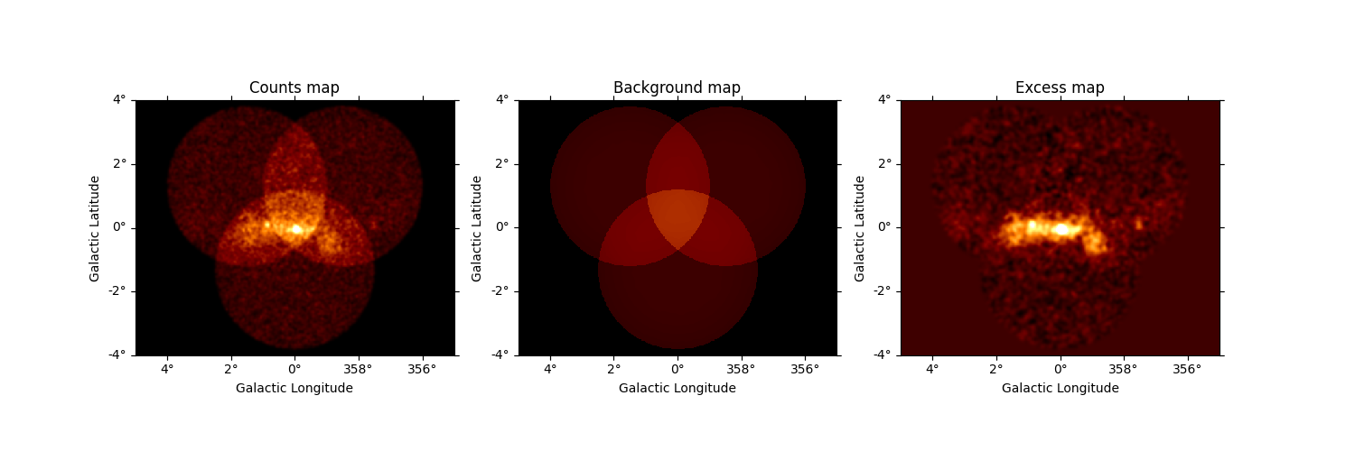
Let’s have a quick look at the images we computed …
fig, (ax1, ax2, ax3) = plt.subplots(
    figsize=(15, 5),
    ncols=3,
    subplot_kw={"projection": geom_image.wcs},
    gridspec_kw={"left": 0.1, "right": 0.9},
)

ax1.set_title("Counts map")
dataset_image.counts.smooth(2).plot(ax=ax1, vmax=5)

ax2.set_title("Background map")
dataset_image.background.plot(ax=ax2, vmax=5)

ax3.set_title("Excess map")
dataset_image.excess.smooth(3).plot(ax=ax3, vmax=2)
plt.show()
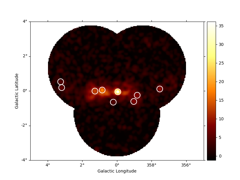
Source Detection#
Use the class TSMapEstimator and function
find_peaks to detect sources on the images.
We search for 0.1 deg sigma gaussian sources in the dataset.
spatial_model = GaussianSpatialModel(sigma="0.05 deg")
spectral_model = PowerLawSpectralModel(index=2)
kernel_model = SkyModel(spatial_model=spatial_model, spectral_model=spectral_model)

ts_image_estimator = TSMapEstimator(
    kernel_model=kernel_model,
    kernel_width="0.5 deg",
    selection_optional=[],
    downsampling_factor=2,
    sum_over_energy_groups=False,
    energy_edges=[0.1, 10] * u.TeV,
)

images_ts = ts_image_estimator.run(stacked)

sources = find_peaks(
    images_ts["sqrt_ts"],
    threshold=5,
    min_distance="0.2 deg",
)
display(sources)
value   x   y      ra       dec
                  deg       deg
------ --- --- --------- ---------
 43.69 252 197 266.42400 -29.00490
22.539 207 202 266.85900 -28.18386
15.977 185 201 267.13594 -27.81751
12.644 373 205 264.79470 -30.97749
 12.28 306 183 266.05018 -30.07215
7.1337  90 209 268.07455 -26.10409
6.1636 405 236 263.78276 -31.18457
5.2418 190  30 270.44708 -29.62765
5.1598  85 227 267.78695 -25.83437
To get the position of the sources, simply
source_pos = SkyCoord(sources["ra"], sources["dec"])
print(source_pos)
<SkyCoord (ICRS): (ra, dec) in deg
    [(266.42399798, -29.00490483), (266.85900392, -28.18385658),
     (267.13594098, -27.81750895), (264.79469899, -30.97749371),
     (266.05017781, -30.07215113), (268.07454639, -26.10409446),
     (263.78276218, -31.18456687), (270.44708387, -29.62765242),
     (267.78695337, -25.83437362)]>
Plot sources on top of significance sky image
fig, ax = plt.subplots(figsize=(8, 6), subplot_kw={"projection": geom_image.wcs})
images_ts["sqrt_ts"].plot(ax=ax, add_cbar=True)

ax.scatter(
    source_pos.ra.deg,
    source_pos.dec.deg,
    transform=ax.get_transform("icrs"),
    color="none",
    edgecolor="white",
    marker="o",
    s=200,
    lw=1.5,
)
plt.show()
Spatial analysis#
See other notebooks for how to run a 3D cube or 2D image based analysis.
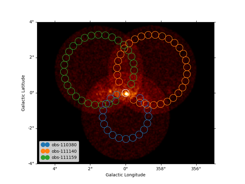
Spectrum#
We’ll run a spectral analysis using the classical reflected regions background estimation method, and using the on-off (often called WSTAT) likelihood function.
target_position = SkyCoord(0, 0, unit="deg", frame="galactic")
on_radius = 0.2 * u.deg
on_region = CircleSkyRegion(center=target_position, radius=on_radius)

exclusion_mask = ~geom.to_image().region_mask([on_region])
exclusion_mask.plot()
plt.show()
Configure spectral analysis
energy_axis = MapAxis.from_energy_bounds(0.1, 40, 40, unit="TeV", name="energy")
energy_axis_true = MapAxis.from_energy_bounds(
    0.05, 100, 200, unit="TeV", name="energy_true"
)

geom = RegionGeom.create(region=on_region, axes=[energy_axis])
dataset_empty = SpectrumDataset.create(geom=geom, energy_axis_true=energy_axis_true)

dataset_maker = SpectrumDatasetMaker(
    containment_correction=False, selection=["counts", "exposure", "edisp"]
)
bkg_maker = ReflectedRegionsBackgroundMaker(exclusion_mask=exclusion_mask)
safe_mask_masker = SafeMaskMaker(methods=["aeff-max"], aeff_percent=10)
Run data reduction
datasets = Datasets()

for observation in observations:
    dataset = dataset_maker.run(
        dataset_empty.copy(name=f"obs-{observation.obs_id}"), observation
    )
    dataset_on_off = bkg_maker.run(dataset, observation)
    dataset_on_off = safe_mask_masker.run(dataset_on_off, observation)
    datasets.append(dataset_on_off)
Plot results
plt.figure(figsize=(8, 6))
ax = dataset_image.counts.smooth("0.03 deg").plot(vmax=8)

on_region.to_pixel(ax.wcs).plot(ax=ax, edgecolor="white")
plot_spectrum_datasets_off_regions(datasets, ax=ax)
plt.show()
Model fit#
The next step is to fit a spectral model, using all data (i.e. a “global” fit, using all energies).
spectral_model = PowerLawSpectralModel(
    index=2, amplitude=1e-11 * u.Unit("cm-2 s-1 TeV-1"), reference=1 * u.TeV
)

model = SkyModel(spectral_model=spectral_model, name="source-gc")

datasets.models = model

fit = Fit()
result = fit.run(datasets=datasets)
print(result)
OptimizeResult

        backend    : minuit
        method     : migrad
        success    : True
        message    : Optimization terminated successfully.
        nfev       : 104
        total stat : 88.36

CovarianceResult

        backend    : minuit
        method     : hesse
        success    : True
        message    : Hesse terminated successfully.
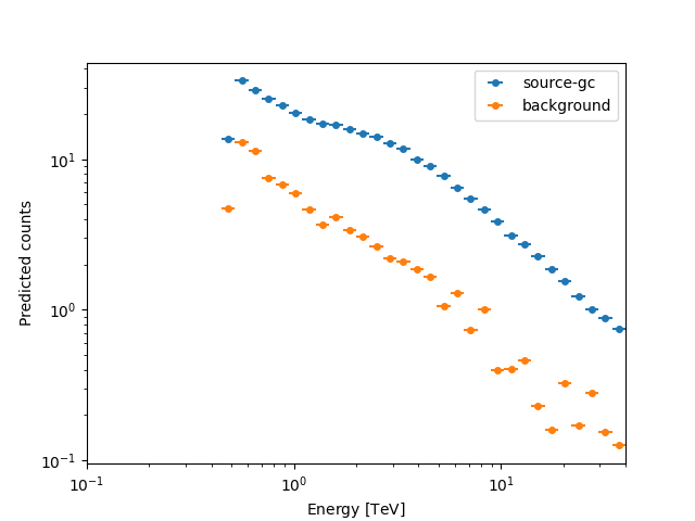
Here we can plot the predicted number of counts for each model and for the background in the dataset. This is especially useful when studying complex field with a lot a sources. There is a function in the visualization sub-package of gammapy that does this automatically.
First we need to stack our datasets.
stacked_dataset = datasets.stack_reduce(name="stacked")
stacked_dataset.models = model

print(stacked_dataset)
SpectrumDatasetOnOff
--------------------

  Name                            : stacked

  Total counts                    : 413
  Total background counts         : 85.43
  Total excess counts             : 327.57

  Predicted counts                : 413.95
  Predicted background counts     : 85.42
  Predicted excess counts         : 328.53

  Exposure min                    : 9.94e+07 m2 s
  Exposure max                    : 2.46e+10 m2 s

  Number of total bins            : 40
  Number of fit bins              : 30

  Fit statistic type              : wstat
  Fit statistic value (-2 log(L)) : 34.70

  Number of models                : 1
  Number of parameters            : 3
  Number of free parameters       : 2

  Component 0: SkyModel

    Name                      : source-gc
    Datasets names            : None
    Spectral model type       : PowerLawSpectralModel
    Spatial  model type       :
    Temporal model type       :
    Parameters:
      index                         :      2.403   +/-    0.06
      amplitude                     :   3.28e-12   +/- 2.3e-13 1 / (TeV s cm2)
      reference             (frozen):      1.000       TeV

    Total counts_off                : 2095
  Acceptance                      : 88
  Acceptance off                  : 2197
Call plot_npred_signal to plot the predicted counts.
/home/runner/work/gammapy-docs/gammapy-docs/gammapy/.tox/build_docs/lib/python3.12/site-packages/gammapy/maps/region/ndmap.py:154: UserWarning: This axis already has a converter set and is updating to a potentially incompatible converter
  ax.errorbar(
Spectral points#
Finally, let’s compute spectral points. The method used is to first choose an energy binning, and then to do a 1-dim likelihood fit / profile to compute the flux and flux error.
# Flux points are computed on stacked datasets
energy_edges = MapAxis.from_energy_bounds("1 TeV", "30 TeV", nbin=5).edges

fpe = FluxPointsEstimator(energy_edges=energy_edges, source="source-gc")
flux_points = fpe.run(datasets=[stacked_dataset])
flux_points.to_table(sed_type="dnde", formatted=True)
Plot#
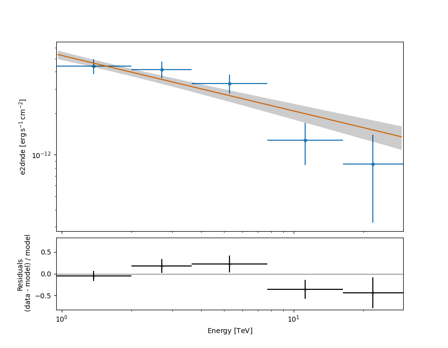
Let’s plot the spectral model and points. You could do it directly, but
for convenience we bundle the model and the flux points in a
FluxPointsDataset:
flux_points_dataset = FluxPointsDataset(data=flux_points, models=model)
flux_points_dataset.plot_fit()
plt.show()
/home/runner/work/gammapy-docs/gammapy-docs/gammapy/.tox/build_docs/lib/python3.12/site-packages/gammapy/modeling/models/spectral.py:649: UserWarning: This axis already has a converter set and is updating to a potentially incompatible converter
  ax.plot(energy.center, flux.quantity[:, 0, 0], **kwargs)
Exercises#
Re-run the analysis above, varying some analysis parameters, e.g.
Select a few other observations
Change the energy band for the map
Change the spectral model for the fit
Change the energy binning for the spectral points
Change the target. Make a sky image and spectrum for your favourite source.
If you don’t know any, the Crab nebula is the “hello world!” analysis of gamma-ray astronomy.
# print('hello world')
# SkyCoord.from_name('crab')
What next?#
This notebook showed an example of a first CTAO analysis with Gammapy, using simulated 1DC data.
Let us know if you have any questions or issues!
Total running time of the script: (0 minutes 11.444 seconds)