Estimation of time variability in a lightcurve

Compute a series of time variability significance estimators for a lightcurve.

Prerequisites

Understanding the light curve estimator, please refer to the Light curves tutorial. For more in-depth explanation on the creation of smaller observations for exploring time variability, refer to the Light curves for flares tutorial.

Context

Frequently, after computing a lightcurve, we need to quantify its variability in the time domain, for example in the case of a flare, burst, decaying light curve in GRBs or heightened activity in general.

There are many ways to define the significance of the variability.

Objective: Estimate the level time variability in a lightcurve through different methods.

Proposed approach

We will start by reading the pre-computed light curve for PKS 2155-304 that is stored in $GAMMAPY_DATA To learn how to compute such an object, see the Light curves for flares tutorial.

This tutorial will demonstrate how to compute different estimates which measure the significance of variability. These estimators range from basic ones that calculate the peak-to-trough variation, to more complex ones like fractional excess and point-to-point fractional variance, which consider the entire light curve. We also show an approach which utilises the change points in Bayesian blocks as indicators of variability.

Setup

As usual, we’ll start with some general imports…

import numpy as np
from astropy.stats import bayesian_blocks
from astropy.time import Time
import matplotlib.pyplot as plt
from gammapy.estimators import FluxPoints
from gammapy.estimators.utils import (
    compute_lightcurve_doublingtime,
    compute_lightcurve_fpp,
    compute_lightcurve_fvar,
)
from gammapy.maps import TimeMapAxis

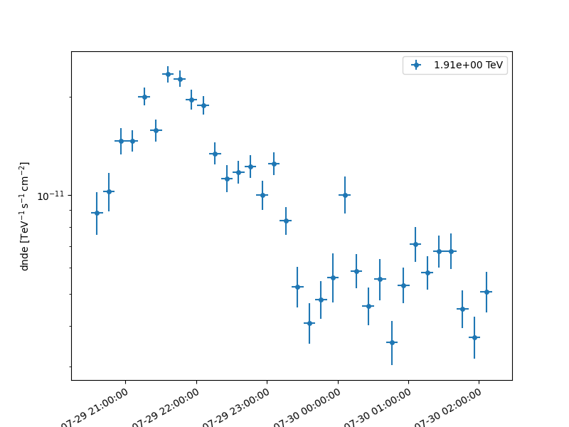
Load the light curve for the PKS 2155-304 flare directly from $GAMMAPY_DATA/estimators.

lc_1d = FluxPoints.read(
    "$GAMMAPY_DATA/estimators/pks2155_hess_lc/pks2155_hess_lc.fits", format="lightcurve"
)

plt.figure(figsize=(8, 6))
lc_1d.plot(marker="o")
plt.show()

Methods to characterize variability

The three methods shown here are:

• amplitude maximum variation

• relative variability amplitude

• variability amplitude.

The amplitude maximum variation is the simplest method to define variability (as described in Boller et al., 2016) as it just computes the level of tension between the lowest and highest measured fluxes in the lightcurve. This estimator requires fully Gaussian errors.

flux = lc_1d.flux.quantity
flux_err = lc_1d.flux_err.quantity

f_mean = np.mean(flux)
f_mean_err = np.mean(flux_err)

f_max = flux.max()
f_max_err = flux_err[flux.argmax()]
f_min = flux.min()
f_min_err = flux_err[flux.argmin()]

amplitude_maximum_variation = (f_max - f_max_err) - (f_min + f_min_err)

amplitude_maximum_significance = amplitude_maximum_variation / np.sqrt(
    f_max_err**2 + f_min_err**2
)

print(amplitude_maximum_significance)

[[[12.41584196]]]

There are other methods based on the peak-to-trough difference to assess the variability in a lightcurve. Here we present as example the relative variability amplitude as presented in Kovalev et al., 2004:

relative_variability_amplitude = (f_max - f_min) / (f_max + f_min)

relative_variability_error = (
    2
    * np.sqrt((f_max * f_min_err) ** 2 + (f_min * f_max_err) ** 2)
    / (f_max + f_min) ** 2
)

relative_variability_significance = (
    relative_variability_amplitude / relative_variability_error
)

print(relative_variability_significance)

[[[19.613114]]]

The variability amplitude as presented in Heidt & Wagner, 1996 is:

variability_amplitude = np.sqrt((f_max - f_min) ** 2 - 2 * f_mean_err**2)

variability_amplitude_100 = 100 * variability_amplitude / f_mean

variability_amplitude_error = (
    100
    * ((f_max - f_min) / (f_mean * variability_amplitude_100 / 100))
    * np.sqrt(
        (f_max_err / f_mean) ** 2
        + (f_min_err / f_mean) ** 2
        + ((np.std(flux, ddof=1) / np.sqrt(len(flux))) / (f_max - f_mean)) ** 2
        * (variability_amplitude_100 / 100) ** 4
    )
)

variability_amplitude_significance = (
    variability_amplitude_100 / variability_amplitude_error
)

print(variability_amplitude_significance)

[[[6.12525306]]]

Fractional excess variance, point-to-point fractional variance and doubling/halving time

The fractional excess variance, as presented by Vaughan et al., 2003, is a simple but effective method to assess the significance of a time variability feature in an object, for example an AGN flare. It is important to note that it requires Gaussian errors to be applicable. The excess variance computation is implemented in utils.

fvar_table = compute_lightcurve_fvar(lc_1d)
print(fvar_table)

    min_energy         max_energy    ...       fvar_err         significance
       TeV                TeV        ...
------------------ ----------------- ... ------------------- ------------------
0.5915030546513255 6.184989894219835 ... 0.01700709977114979 33.082691868487906

A similar estimator is the point-to-point fractional variance, as defined by Edelson et al., 2002, which samples the lightcurve on smaller time granularity. In general, the point-to-point fractional variance being higher than the fractional excess variance is indicative of the presence of very short timescale variability.

fpp_table = compute_lightcurve_fpp(lc_1d)
print(fpp_table)

    min_energy         max_energy    ...       fpp_err          significance
       TeV                TeV        ...
------------------ ----------------- ... -------------------- ----------------
0.5915030546513255 6.184989894219835 ... 0.017442925431194484 15.2995484265169

The characteristic doubling and halving time of the light curve, as introduced by Brown, 2013, can also be computed. This provides information on the shape of the variability feature, in particular how quickly it rises and falls.

dtime_table = compute_lightcurve_doublingtime(lc_1d, flux_quantity="flux")
print(dtime_table)

    min_energy         max_energy    ...    halving_err       halving_coord
       TeV                TeV        ...         s
------------------ ----------------- ... ------------------ -----------------
0.5915030546513255 6.184989894219835 ... 20.935826709880043 53946.00422666667

Bayesian blocks

The presence of temporal variability in a lightcurve can be assessed by using bayesian blocks (Scargle et al., 2013). A good and simple-to-use implementation of the algorithm is found in astropy.stats.bayesian_blocks. This implementation uses Gaussian statistics, as opposed to the first introductory paper which is based on Poissonian statistics.

By passing the flux and error on the flux as measures to the method we can obtain the list of optimal bin edges defined by the bayesian blocks algorithm.

time = lc_1d.geom.axes["time"].time_mid.mjd

bayesian_edges = bayesian_blocks(
    t=time, x=flux.flatten(), sigma=flux_err.flatten(), fitness="measures"
)

The result giving a significance estimation for variability in the lightcurve is the number of change points, i.e. the number of internal bin edges: if at least one change point is identified by the algorithm, there is significant variability.

ncp = len(bayesian_edges) - 2
print(ncp)

7

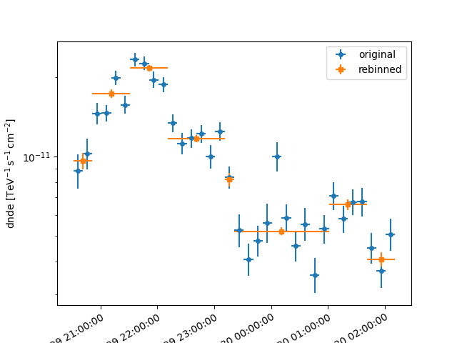
We can rebin the lightcurve to compute the one expected with bayesian edges First, we adjust the first and last bins of the bayesian_edges to coincide with the original light curve start and end points.

# create a new axis
axis_original = lc_1d.geom.axes["time"]
bayesian_edges[0] = axis_original.time_edges[0].value
bayesian_edges[-1] = axis_original.time_edges[-1].value
edges = Time(bayesian_edges, format="mjd", scale=axis_original.reference_time.scale)
axis_new = TimeMapAxis.from_time_edges(edges[:-1], edges[1:])

# rebin the lightcurve
resample = lc_1d.resample_axis(axis_new)

# plot the new lightcurve on top of the old one
ax = lc_1d.plot(label="original")
resample.plot(ax=ax, marker="s", label="rebinned")
plt.legend()

<matplotlib.legend.Legend object at 0x7f3bc80bac70>