Note
Go to the end to download the full example code. or to run this example in your browser via Binder
Source catalogs#
Access and explore thew most common gamma-ray source catalogs.
Introduction#
catalog provides convenient access to common gamma-ray
source catalogs. This module is mostly independent of the rest of
Gammapy. Typically, you use it to compare new analyses against catalog
results, e.g. overplot the spectral model, or compare the source
position.
Moreover, as creating a source model and flux points for a given catalog
from the FITS table is tedious, catalog has this already
implemented. So you can create initial source models for your analyses.
This is very common for Fermi-LAT, to start with a catalog model. For
TeV analysis, especially in crowded Galactic regions, using the HGPS,
gamma-cat or 2HWC catalog in this way can also be useful.
In this tutorial you will learn how to:
List available catalogs
Load a catalog
Access the source catalog table data
Select a catalog subset or a single source
Get source spectral and spatial models
Get flux points (if available)
Get lightcurves (if available)
Access the source catalog table data
Pretty-print the source information
In this tutorial we will show examples using the following catalogs:
All catalog and source classes work the same, as long as some
information is available. E.g. trying to access a lightcurve from a
catalog and source that does not have that information will return
None.
Further information is available at catalog.
import numpy as np
import astropy.units as u

# %matplotlib inline
import matplotlib.pyplot as plt
from IPython.display import display
from gammapy.catalog import SourceCatalog4FGL
from gammapy.catalog import CATALOG_REGISTRY
Check setup#
from gammapy.utils.check import check_tutorials_setup

check_tutorials_setup()
System:

        python_executable      : /home/runner/work/gammapy-docs/gammapy-docs/gammapy/.tox/build_docs/bin/python
        python_version         : 3.9.22
        machine                : x86_64
        system                 : Linux


Gammapy package:

        version                : 2.0.dev1224+g83b25692c
        path                   : /home/runner/work/gammapy-docs/gammapy-docs/gammapy/.tox/build_docs/lib/python3.9/site-packages/gammapy


Other packages:

        numpy                  : 1.26.4
        scipy                  : 1.13.1
        astropy                : 6.0.1
        regions                : 0.8
        click                  : 8.1.8
        yaml                   : 6.0.2
        IPython                : 8.18.1
        jupyterlab             : not installed
        matplotlib             : 3.9.4
        pandas                 : not installed
        healpy                 : 1.17.3
        iminuit                : 2.31.1
        sherpa                 : 4.16.1
        naima                  : 0.10.0
        emcee                  : 3.1.6
        corner                 : 2.2.3
        ray                    : 2.46.0


Gammapy environment variables:

        GAMMAPY_DATA           : /home/runner/work/gammapy-docs/gammapy-docs/gammapy-datasets/dev
List available catalogs#
catalog contains a catalog registry CATALOG_REGISTRY,
which maps catalog names (e.g. “3fhl”) to catalog classes
(e.g. SourceCatalog3FHL).
print(CATALOG_REGISTRY)
Registry
--------

SourceCatalogGammaCat: gamma-cat
SourceCatalogHGPS    : hgps
SourceCatalog2HWC    : 2hwc
SourceCatalog3FGL    : 3fgl
SourceCatalog4FGL    : 4fgl
SourceCatalog2FHL    : 2fhl
SourceCatalog3FHL    : 3fhl
SourceCatalog3PC     : 3PC
SourceCatalog3HWC    : 3hwc
SourceCatalog2PC     : 2PC
SourceCatalog1LHAASO : 1LHAASO
Load catalogs#
If you have run gammapy download datasets or
gammapy download tutorials, you have a copy of the catalogs as FITS
files in $GAMMAPY_DATA/catalogs, and that is the default location
where catalog loads from.
# # # !ls -1 $GAMMAPY_DATA/catalogs
# # # !ls -1 $GAMMAPY_DATA/catalogs/fermi
So a catalog can be loaded directly from its corresponding class
catalog = SourceCatalog4FGL()
print("Number of sources :", len(catalog.table))
Number of sources : 7195
Note that it loads the default catalog from $GAMMAPY_DATA/catalogs,
you could pass a different filename when creating the catalog. For
example here we load an older version of 4FGL catalog:
catalog = SourceCatalog4FGL("$GAMMAPY_DATA/catalogs/fermi/gll_psc_v20.fit.gz")
print("Number of sources :", len(catalog.table))
Number of sources : 5066
Alternatively you can load a catalog by name via
CATALOG_REGISTRY.get_cls(name)() (note the () to instantiate a
catalog object from the catalog class - only this will load the catalog
and be useful), or by importing the catalog class
(e.g. SourceCatalog3FGL) directly. The two ways are equivalent, the
result will be the same.
# FITS file is loaded
catalog = CATALOG_REGISTRY.get_cls("3fgl")()
print(catalog)
SourceCatalog3FGL:
    name: 3fgl
    description: LAT 4-year point source catalog
    sources: 3034
Let’s load the source catalogs we will use throughout this tutorial
catalog_gammacat = CATALOG_REGISTRY.get_cls("gamma-cat")()
catalog_3fhl = CATALOG_REGISTRY.get_cls("3fhl")()
catalog_4fgl = CATALOG_REGISTRY.get_cls("4fgl")()
catalog_hgps = CATALOG_REGISTRY.get_cls("hgps")()
Catalog table#
Source catalogs are given as FITS files that contain one or multiple
tables.
However, you can also access the underlying astropy.table.Table for
a catalog, and the row data as a Python dict. This can be useful if
you want to do something that is not pre-scripted by the
SourceCatalog classes, such as e.g. selecting sources by sky
position or association class, or accessing special source information.
print(type(catalog_3fhl.table))
<class 'astropy.table.table.Table'>
print(len(catalog_3fhl.table))
1556
display(catalog_3fhl.table[:3][["Source_Name", "RAJ2000", "DEJ2000"]])
   Source_Name     RAJ2000  DEJ2000
                     deg      deg
------------------ -------- --------
3FHL J0001.2-0748    0.3107  -7.8075
3FHL J0001.9-4155    0.4849 -41.9303
3FHL J0002.1-6728    0.5283 -67.4825
Note that the catalogs object include a helper property that gives
directly the sources positions as a SkyCoord object (we will show an
usage example in the following).
print(catalog_3fhl.positions[:3])
<SkyCoord (ICRS): (ra, dec) in deg
    [(0.31067517,  -7.8075185), (0.4848653 , -41.93026  ),
     (0.52826166, -67.48248  )]>
Source object#
Select a source#
The catalog entries for a single source are represented by a
SourceCatalogObject. In order to select a source object index into
the catalog using [], with a catalog table row index (zero-based,
first row is [0]), or a source name. If a name is given, catalog
table columns with source names and association names (“ASSOC1” in the
example below) are searched top to bottom. There is no name resolution
web query.
source = catalog_4fgl[49]
print(source)
*** Basic info ***

Catalog row index (zero-based) : 49
Source name          : 4FGL J0008.9+2509
Extended name        :
Associations     :
ASSOC_PROB_BAY   : 0.000
ASSOC_PROB_LR    : 0.000
Class1           :
Class2           :
TeVCat flag      : N

*** Other info ***

Significance (100 MeV - 1 TeV)   : 4.126
Npred                            : 571.6

Other flags          : 0

*** Position info ***

RA                   : 2.236 deg
DEC                  : 25.154 deg
GLON                 : 110.915 deg
GLAT                 : -36.725 deg

Semimajor (68%)      : 0.1553 deg
Semiminor (68%)      : 0.1211 deg
Position angle (68%) : -6.18 deg
Semimajor (95%)      : 0.2518 deg
Semiminor (95%)      : 0.1963 deg
Position angle (95%) : -6.18 deg
ROI number           : 1344

*** Spectral info ***

Spectrum type                                 : PowerLaw
Detection significance (100 MeV - 1 TeV)      : 4.126
Pivot energy                                  : 407 MeV
Spectral index                                : 2.889 +- 0.166
Flux Density at pivot energy                  : 1.9e-12 +- 3.85e-13 cm-2 MeV-1 s-1
Integral flux (1 - 100 GeV)                   : 7.48e-11 +- 2.34e-11 cm-2 s-1
Energy flux (100 MeV - 100 GeV)               : 1.97e-12 +- 4.11e-13 erg cm-2 s-1

*** Spectral points ***

  e_min       e_max        flux     flux_errn   flux_errp      e2dnde     e2dnde_errn   e2dnde_errp  is_ul   flux_ul     e2dnde_ul   sqrt_ts
   MeV         MeV     1 / (s cm2) 1 / (s cm2) 1 / (s cm2) erg / (s cm2) erg / (s cm2) erg / (s cm2)       1 / (s cm2) erg / (s cm2)
---------- ----------- ----------- ----------- ----------- ------------- ------------- ------------- ----- ----------- ------------- -------
    50.000     100.000   1.601e-09         nan   1.348e-08     2.477e-13           nan     2.086e-12  True   2.856e-08     4.419e-12   0.015
   100.000     300.000   1.539e-09         nan   2.036e-09     3.398e-13           nan     4.498e-13  True   5.611e-09     1.239e-12   0.713
   300.000    1000.000   7.810e-10   2.102e-10   2.147e-10     4.852e-13     1.306e-13     1.334e-13 False         nan           nan   3.905
  1000.000    3000.000   7.227e-11   3.036e-11   3.307e-11     1.596e-13     6.706e-14     7.305e-14 False         nan           nan   2.585
  3000.000   10000.000   3.177e-12         nan   9.940e-12     1.974e-14           nan     6.175e-14  True   2.306e-11     1.432e-13   0.400
 10000.000   30000.000   8.771e-15         nan   4.719e-12     1.938e-16           nan     1.042e-13  True   9.447e-12     2.087e-13   0.000
 30000.000  100000.000   6.142e-16         nan   2.774e-12     3.816e-17           nan     1.723e-13  True   5.548e-12     3.447e-13   0.000
100000.000 1000000.000   9.286e-16         nan   3.149e-12     1.211e-16           nan     4.107e-13  True   6.299e-12     8.215e-13   0.000
*** Lightcurve info ***

Lightcurve measured in the energy band: 100 MeV - 100 GeV

Variability index : 20.426

No peak measured for this source.
print(source.row_index, source.name)
49 4FGL J0008.9+2509
source = catalog_4fgl["4FGL J0010.8-2154"]
print(source.row_index, source.name)
64 4FGL J0010.8-2154
print(source.data["ASSOC1"])
PKS 0008-222
source = catalog_4fgl["PKS 0008-222"]
print(source.row_index, source.name)
64 4FGL J0010.8-2154
Note that you can also do a for source in catalog loop, to find or
process sources of interest.
Source information#
The source objects have a data property that contains the
information of the catalog row corresponding to the source.
print(source.data["Npred"])
336.59976
60.28118133544922 deg -79.40050506591797 deg
As for the catalog object, the source object has a position
property.
print(source.position.galactic)
<SkyCoord (Galactic): (l, b) in deg
    (60.28120079, -79.40051035)>
Select a catalog subset#
The catalog objects support selection using boolean arrays (of the same length), so one can create a new catalog as a subset of the main catalog that verify a set of conditions.
In the next example we selection only few of the brightest sources brightest sources in the 100 to 200 GeV energy band.
mask_bright = np.zeros(len(catalog_3fhl.table), dtype=bool)
for k, source in enumerate(catalog_3fhl):
    flux = source.spectral_model().integral(100 * u.GeV, 200 * u.GeV).to("cm-2 s-1")
    if flux > 1e-10 * u.Unit("cm-2 s-1"):
        mask_bright[k] = True
        print(f"{source.row_index:<7d} {source.name:20s} {flux:.3g}")
352     3FHL J0534.5+2201    2.99e-10 1 / (s cm2)
553     3FHL J0851.9-4620e   1.24e-10 1 / (s cm2)
654     3FHL J1036.3-5833e   1.57e-10 1 / (s cm2)
691     3FHL J1104.4+3812    3.34e-10 1 / (s cm2)
1111    3FHL J1653.8+3945    1.27e-10 1 / (s cm2)
1219    3FHL J1824.5-1351e   1.77e-10 1 / (s cm2)
1361    3FHL J2028.6+4110e   1.75e-10 1 / (s cm2)
SourceCatalog3FHL:
    name: 3fhl
    description: LAT third high-energy source catalog
    sources: 7
print(catalog_3fhl_bright.table["Source_Name"])
   Source_Name
------------------
3FHL J0534.5+2201
3FHL J0851.9-4620e
3FHL J1036.3-5833e
3FHL J1104.4+3812
3FHL J1653.8+3945
3FHL J1824.5-1351e
3FHL J2028.6+4110e
Similarly we can select only sources within a region of interest. Here
for example we use the position property of the catalog object to
select sources within 5 degrees from “PKS 0008-222”:
source = catalog_4fgl["PKS 0008-222"]
mask_roi = source.position.separation(catalog_4fgl.positions) < 5 * u.deg

catalog_4fgl_roi = catalog_4fgl[mask_roi]
print("Number of sources :", len(catalog_4fgl_roi.table))
Number of sources : 16
Source models#
The SourceCatalogObject classes have a
sky_model() model which creates a
SkyModel object, with model parameter values
and parameter errors from the catalog filled in.
In most cases, the spectral_model() method provides the
SpectralModel part of the sky model, and the
spatial_model() method the SpatialModel
part individually.
We use the SourceCatalog3FHL for the examples in
this section.
source = catalog_4fgl["PKS 2155-304"]

model = source.sky_model()
print(model)
SkyModel

  Name                      : 4FGL J2158.8-3013
  Datasets names            : None
  Spectral model type       : LogParabolaSpectralModel
  Spatial  model type       : PointSpatialModel
  Temporal model type       :
  Parameters:
    amplitude                     :   1.26e-11   +/- 1.3e-13 1 / (MeV s cm2)
    reference             (frozen):   1160.973       MeV
    alpha                         :      1.773   +/-    0.01
    beta                          :      0.042   +/-    0.00
    lon_0                         :    329.714   +/-    0.00 deg
    lat_0                         :    -30.225   +/-    0.00 deg
print(model.spatial_model)
PointSpatialModel

type  name    value    unit   error      min        max    frozen link prior
---- ----- ----------- ---- --------- ---------- --------- ------ ---- -----
     lon_0  3.2971e+02  deg 3.735e-03        nan       nan  False
     lat_0 -3.0225e+01  deg 3.227e-03 -9.000e+01 9.000e+01  False
print(model.spectral_model)
LogParabolaSpectralModel

type    name     value         unit        error   min max frozen link prior
---- --------- ---------- -------------- --------- --- --- ------ ---- -----
     amplitude 1.2591e-11 MeV-1 s-1 cm-2 1.317e-13 nan nan  False
     reference 1.1610e+03            MeV 0.000e+00 nan nan   True
         alpha 1.7733e+00                1.029e-02 nan nan  False
          beta 4.1893e-02                3.743e-03 nan nan  False
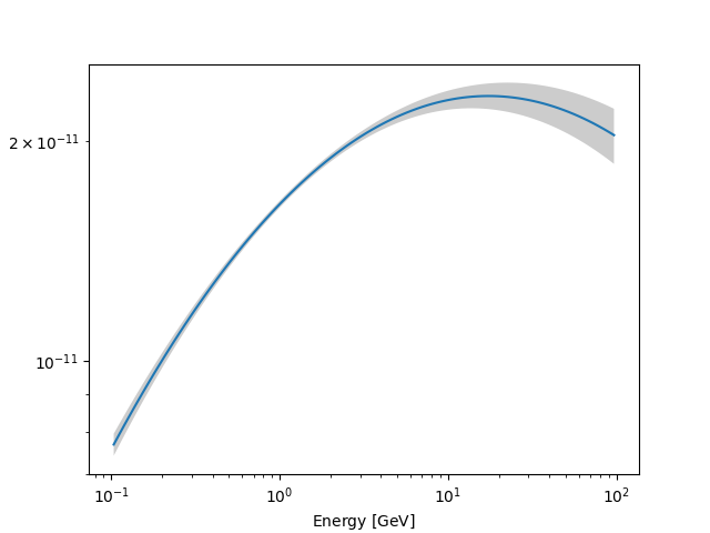
energy_bounds = (100 * u.MeV, 100 * u.GeV)
opts = dict(sed_type="e2dnde", yunits=u.Unit("TeV cm-2 s-1"))
model.spectral_model.plot(energy_bounds, **opts)
model.spectral_model.plot_error(energy_bounds, **opts)
plt.show()
You can create initial source models for your analyses using the
to_models() method of the catalog objects. Here for example we
create a Models object from the 4FGL catalog subset we previously
defined:
Models

Component 0: SkyModel

  Name                      : 4FGL J0001.8-2153
  Datasets names            : None
  Spectral model type       : PowerLawSpectralModel
  Spatial  model type       : PointSpatialModel
  Temporal model type       :
  Parameters:
    index                         :      1.906   +/-    0.19
    amplitude                     :   4.47e-15   +/- 1.2e-15 1 / (MeV s cm2)
    reference             (frozen):   4281.748       MeV
    lon_0                         :      0.465   +/-    0.04 deg
    lat_0                         :    -21.886   +/-    0.05 deg

Component 1: SkyModel

  Name                      : 4FGL J0003.3-1928
  Datasets names            : None
  Spectral model type       : LogParabolaSpectralModel
  Spatial  model type       : PointSpatialModel
  Temporal model type       :
  Parameters:
    amplitude                     :   4.73e-13   +/- 4.5e-14 1 / (MeV s cm2)
    reference             (frozen):   1064.702       MeV
    alpha                         :      2.136   +/-    0.12
    beta                          :      0.211   +/-    0.08
    lon_0                         :      0.846   +/-    0.03 deg
    lat_0                         :    -19.468   +/-    0.03 deg

Component 2: SkyModel

  Name                      : 4FGL J0006.3-1813
  Datasets names            : None
  Spectral model type       : PowerLawSpectralModel
  Spatial  model type       : PointSpatialModel
  Temporal model type       :
  Parameters:
    index                         :      2.278   +/-    0.21
    amplitude                     :   2.94e-14   +/- 7.3e-15 1 / (MeV s cm2)
    reference             (frozen):   1808.240       MeV
    lon_0                         :      1.578   +/-    0.03 deg
    lat_0                         :    -18.229   +/-    0.03 deg

Component 3: SkyModel

  Name                      : 4FGL J0008.4-2339
  Datasets names            : None
  Spectral model type       : PowerLawSpectralModel
  Spatial  model type       : PointSpatialModel
  Temporal model type       :
  Parameters:
    index                         :      1.810   +/-    0.10
    amplitude                     :   1.01e-14   +/- 1.5e-15 1 / (MeV s cm2)
    reference             (frozen):   4481.370       MeV
    lon_0                         :      2.111   +/-    0.02 deg
    lat_0                         :    -23.651   +/-    0.02 deg

Component 4: SkyModel

  Name                      : 4FGL J0010.2-2431
  Datasets names            : None
  Spectral model type       : PowerLawSpectralModel
  Spatial  model type       : PointSpatialModel
  Temporal model type       :
  Parameters:
    index                         :      2.176   +/-    0.18
    amplitude                     :   1.98e-14   +/- 4.9e-15 1 / (MeV s cm2)
    reference             (frozen):   2131.147       MeV
    lon_0                         :      2.560   +/-    0.03 deg
    lat_0                         :    -24.524   +/-    0.04 deg

Component 5: SkyModel

  Name                      : 4FGL J0010.8-2154
  Datasets names            : None
  Spectral model type       : PowerLawSpectralModel
  Spatial  model type       : PointSpatialModel
  Temporal model type       :
  Parameters:
    index                         :      2.344   +/-    0.15
    amplitude                     :   8.39e-14   +/- 1.6e-14 1 / (MeV s cm2)
    reference             (frozen):   1299.988       MeV
    lon_0                         :      2.717   +/-    0.05 deg
    lat_0                         :    -21.900   +/-    0.05 deg

Component 6: SkyModel

  Name                      : 4FGL J0013.9-1854
  Datasets names            : None
  Spectral model type       : PowerLawSpectralModel
  Spatial  model type       : PointSpatialModel
  Temporal model type       :
  Parameters:
    index                         :      1.905   +/-    0.08
    amplitude                     :   2.58e-14   +/- 2.9e-15 1 / (MeV s cm2)
    reference             (frozen):   3299.164       MeV
    lon_0                         :      3.480   +/-    0.02 deg
    lat_0                         :    -18.912   +/-    0.02 deg

Component 7: SkyModel

  Name                      : 4FGL J0021.5-2221
  Datasets names            : None
  Spectral model type       : LogParabolaSpectralModel
  Spatial  model type       : PointSpatialModel
  Temporal model type       :
  Parameters:
    amplitude                     :   6.85e-13   +/- 1.5e-13 1 / (MeV s cm2)
    reference             (frozen):    620.905       MeV
    alpha                         :      2.662   +/-    0.23
    beta                          :      0.268   +/-    0.16
    lon_0                         :      5.383   +/-    0.06 deg
    lat_0                         :    -22.358   +/-    0.08 deg

Component 8: SkyModel

  Name                      : 4FGL J0021.5-2552
  Datasets names            : None
  Spectral model type       : LogParabolaSpectralModel
  Spatial  model type       : PointSpatialModel
  Temporal model type       :
  Parameters:
    amplitude                     :   8.68e-13   +/- 5.4e-14 1 / (MeV s cm2)
    reference             (frozen):    969.357       MeV
    alpha                         :      2.009   +/-    0.07
    beta                          :      0.082   +/-    0.03
    lon_0                         :      5.391   +/-    0.01 deg
    lat_0                         :    -25.868   +/-    0.01 deg

Component 9: SkyModel

  Name                      : 4FGL J0022.1-1854
  Datasets names            : None
  Spectral model type       : LogParabolaSpectralModel
  Spatial  model type       : PointSpatialModel
  Temporal model type       :
  Parameters:
    amplitude                     :   3.88e-13   +/- 2.4e-14 1 / (MeV s cm2)
    reference             (frozen):   1482.670       MeV
    alpha                         :      1.788   +/-    0.07
    beta                          :      0.101   +/-    0.03
    lon_0                         :      5.535   +/-    0.01 deg
    lat_0                         :    -18.907   +/-    0.01 deg

Component 10: SkyModel

  Name                      : 4FGL J0025.0-2320
  Datasets names            : None
  Spectral model type       : PowerLawSpectralModel
  Spatial  model type       : PointSpatialModel
  Temporal model type       :
  Parameters:
    index                         :      2.180   +/-    0.20
    amplitude                     :   1.36e-14   +/- 3.7e-15 1 / (MeV s cm2)
    reference             (frozen):   2399.210       MeV
    lon_0                         :      6.268   +/-    0.04 deg
    lat_0                         :    -23.338   +/-    0.05 deg

Component 11: SkyModel

  Name                      : 4FGL J0025.2-2231
  Datasets names            : None
  Spectral model type       : PowerLawSpectralModel
  Spatial  model type       : PointSpatialModel
  Temporal model type       :
  Parameters:
    index                         :      2.147   +/-    0.25
    amplitude                     :   6.93e-15   +/- 2.1e-15 1 / (MeV s cm2)
    reference             (frozen):   3071.779       MeV
    lon_0                         :      6.303   +/-    0.03 deg
    lat_0                         :    -22.533   +/-    0.03 deg

Component 12: SkyModel

  Name                      : 4FGL J0031.0-2327
  Datasets names            : None
  Spectral model type       : LogParabolaSpectralModel
  Spatial  model type       : PointSpatialModel
  Temporal model type       :
  Parameters:
    amplitude                     :   1.10e-13   +/- 1.7e-14 1 / (MeV s cm2)
    reference             (frozen):   1686.153       MeV
    alpha                         :      1.841   +/-    0.22
    beta                          :      0.551   +/-    0.18
    lon_0                         :      7.756   +/-    0.04 deg
    lat_0                         :    -23.458   +/-    0.05 deg

Component 13: SkyModel

  Name                      : 4FGL J2357.7-1937
  Datasets names            : None
  Spectral model type       : PowerLawSpectralModel
  Spatial  model type       : PointSpatialModel
  Temporal model type       :
  Parameters:
    index                         :      2.220   +/-    0.19
    amplitude                     :   2.59e-14   +/- 6.2e-15 1 / (MeV s cm2)
    reference             (frozen):   1978.430       MeV
    lon_0                         :    359.430   +/-    0.04 deg
    lat_0                         :    -19.619   +/-    0.04 deg

Component 14: SkyModel

  Name                      : 4FGL J2358.5-1808
  Datasets names            : None
  Spectral model type       : LogParabolaSpectralModel
  Spatial  model type       : PointSpatialModel
  Temporal model type       :
  Parameters:
    amplitude                     :   1.60e-13   +/- 1.3e-14 1 / (MeV s cm2)
    reference             (frozen):   1980.032       MeV
    alpha                         :      1.783   +/-    0.09
    beta                          :      0.074   +/-    0.03
    lon_0                         :    359.639   +/-    0.01 deg
    lat_0                         :    -18.141   +/-    0.01 deg

Component 15: SkyModel

  Name                      : 4FGL J2359.3-2049
  Datasets names            : None
  Spectral model type       : PowerLawSpectralModel
  Spatial  model type       : PointSpatialModel
  Temporal model type       :
  Parameters:
    index                         :      1.928   +/-    0.07
    amplitude                     :   4.24e-14   +/- 3.9e-15 1 / (MeV s cm2)
    reference             (frozen):   2930.842       MeV
    lon_0                         :    359.836   +/-    0.02 deg
    lat_0                         :    -20.819   +/-    0.02 deg
Specificities of the HGPS catalog#
Using the to_models() method for the
SourceCatalogHGPS will return only the models
components of the sources retained in the main catalog, several
candidate objects appears only in the Gaussian components table (see
section 4.9 of the HGPS paper, https://arxiv.org/abs/1804.02432). To
access these components you can do the following:
discarded_ind = np.where(
    ["Discarded" in _ for _ in catalog_hgps.table_components["Component_Class"]]
)[0]
discarded_table = catalog_hgps.table_components[discarded_ind]
There is no spectral model available for these components but you can access their spatial models:
discarded_spatial = [
    catalog_hgps.gaussian_component(idx).spatial_model() for idx in discarded_ind
]
In addition to the source components the HGPS catalog include a large
scale diffuse component built by fitting a gaussian model in a sliding
window along the Galactic plane. Information on this model can be
accessed via the properties table_large_scale_component and
large_scale_component of SourceCatalogHGPS.
# here we show the 5 first elements of the table
display(catalog_hgps.table_large_scale_component[:5])
# you can also try :
# help(catalog_hgps.large_scale_component)
   GLON       GLAT   GLAT_Err ... Surface_Brightness_Err  Width   Width_Err
   deg        deg      deg    ...     1 / (s sr cm2)       deg       deg
---------- --------- -------- ... ---------------------- -------- ---------
270.000000  0.205357 0.251932 ...           4.064108e-10 0.269385  0.137990
272.959198 -0.120154 0.058201 ...           7.346488e-10 0.088742  0.041882
275.918365 -0.095232 0.089881 ...           6.117877e-10 0.167219  0.111797
278.877563 -0.257642 0.065071 ...           5.230542e-10 0.156525  0.056130
281.836731 -0.283487 0.066442 ...           4.336444e-10 0.205192  0.049676
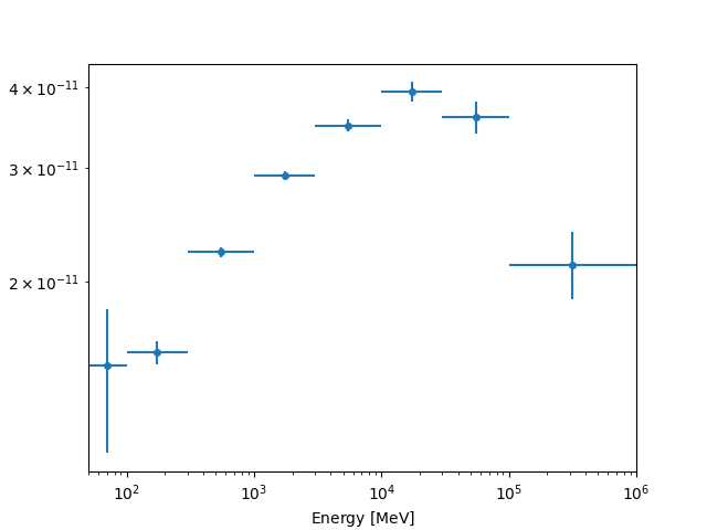
Flux points#
The flux points are available via the flux_points property as a
FluxPoints object.
source = catalog_4fgl["PKS 2155-304"]
flux_points = source.flux_points


print(flux_points)
FluxPoints
----------

  geom                   : RegionGeom
  axes                   : ['lon', 'lat', 'energy']
  shape                  : (1, 1, 8)
  quantities             : ['norm', 'norm_errp', 'norm_errn', 'norm_ul', 'sqrt_ts', 'is_ul']
  ref. model             : lp
  n_sigma                : 1
  n_sigma_ul             : 2
  sqrt_ts_threshold_ul   : 1
  sed type init          : flux
display(flux_points.to_table(sed_type="flux"))
      e_ref              e_min              e_max        ...  sqrt_ts  is_ul
       MeV                MeV                MeV         ...
------------------ ------------------ ------------------ ... --------- -----
 70.71067811865478  49.99999999999999 100.00000000000004 ... 3.1173775 False
173.20508075688775 100.00000000000004 299.99999999999994 ... 25.332525 False
  547.722557505166 299.99999999999994  999.9999999999998 ...  97.62258 False
1732.0508075688763  999.9999999999998 2999.9999999999977 ... 141.84529 False
 5477.225575051666 2999.9999999999977  10000.00000000001 ... 135.62503 False
 17320.50807568877  10000.00000000001 30000.000000000007 ... 97.068245 False
54772.255750516626 30000.000000000007 100000.00000000001 ...  62.05227 False
 316227.7660168382 100000.00000000001  999999.9999999995 ... 31.402712 False
flux_points.plot(sed_type="e2dnde")
plt.show()
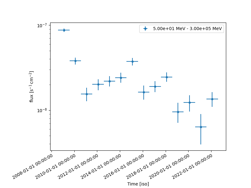
Lightcurves#
The Fermi catalogs contain lightcurves for each source. It is available
via the source.lightcurve method as a
FluxPoints object with a time axis.
lightcurve = catalog_4fgl["4FGL J0349.8-2103"].lightcurve()

print(lightcurve)
FluxPoints
----------

  geom                   : RegionGeom
  axes                   : ['lon', 'lat', 'energy', 'time']
  shape                  : (1, 1, 1, 14)
  quantities             : ['norm', 'norm_errp', 'norm_errn', 'norm_ul', 'ts']
  ref. model             : lp
  n_sigma                : 1
  n_sigma_ul             : 2
  sqrt_ts_threshold_ul   : 1
  sed type init          : flux
display(lightcurve.to_table(format="lightcurve", sed_type="flux"))
     time_min           time_max            e_ref        ...  sqrt_ts  is_ul
                                             MeV         ...
------------------ ------------------ ------------------ ... --------- -----
 54682.65603794185 55045.301668796295 3872.9833462074166 ... 30.809505 False
55045.301668796295  55410.57944657408 3872.9833462074166 ... 14.118355 False
 55410.57944657408  55775.85722435185 3872.9833462074166 ... 6.6116853 False
 55775.85722435185  56141.13500212963 3872.9833462074166 ...  8.432878 False
 56141.13500212963 56506.412779907405 3872.9833462074166 ...  8.800932 False
56506.412779907405 56871.690557685186 3872.9833462074166 ...  9.687685 False
56871.690557685186  57236.96833546296 3872.9833462074166 ... 13.500249 False
 57236.96833546296  57602.24611324074 3872.9833462074166 ...  6.146472 False
 57602.24611324074  57967.52389101852 3872.9833462074166 ...  8.539397 False
 57967.52389101852 58332.801668796295 3872.9833462074166 ...   9.76739 False
58332.801668796295  58698.07944657408 3872.9833462074166 ...  4.498784 False
 58698.07944657408  59063.35722435185 3872.9833462074166 ... 5.3674884 False
 59063.35722435185  59428.63500212963 3872.9833462074166 ... 2.8593054 False
 59428.63500212963 59793.912779907405 3872.9833462074166 ...  6.248122 False
plt.figure(figsize=(8, 6))
plt.subplots_adjust(bottom=0.2, left=0.2)
lightcurve.plot()
plt.show()
Pretty-print source information#
A source object has a nice string representation that you can print.
source = catalog_hgps["MSH 15-52"]
print(source)
*** Basic info ***

Catalog row index (zero-based) : 18
Source name          : HESS J1514-591
Analysis reference   : HGPS
Source class         : PWN
Identified object    : MSH 15-52
Gamma-Cat id         : 79


*** Info from map analysis ***

RA                   :  228.499 deg = 15h14m00s
DEC                  :  -59.161 deg = -59d09m41s
GLON                 :  320.315 +/- 0.008 deg
GLAT                 :   -1.188 +/- 0.007 deg
Position Error (68%) : 0.020 deg
Position Error (95%) : 0.033 deg
ROI number           : 13
Spatial model        : 3-Gaussian
Spatial components   : HGPSC 023, HGPSC 024, HGPSC 025
TS                   : 1763.4
sqrt(TS)             : 42.0
Size                 : 0.145 +/- 0.026 (UL: 0.000) deg
R70                  : 0.215 deg
RSpec                : 0.215 deg
Total model excess   : 3502.8
Excess in RSpec      : 2440.5
Model Excess in RSpec : 2414.3
Background in RSpec  : 1052.5
Livetime             : 41.4 hours
Energy threshold     : 0.61 TeV
Source flux (>1 TeV) : (6.434 +/- 0.211) x 10^-12 cm^-2 s^-1 = (28.47 +/- 0.94) % Crab

Fluxes in RSpec (> 1 TeV):
Map measurement                : 4.552 x 10^-12 cm^-2 s^-1 = 20.14 % Crab
Source model                   : 4.505 x 10^-12 cm^-2 s^-1 = 19.94 % Crab
Other component model          : 0.000 x 10^-12 cm^-2 s^-1 =  0.00 % Crab
Large scale component model    : 0.000 x 10^-12 cm^-2 s^-1 =  0.00 % Crab
Total model                    : 4.505 x 10^-12 cm^-2 s^-1 = 19.94 % Crab
Containment in RSpec                :  70.0 %
Contamination in RSpec              :   0.0 %
Flux correction (RSpec -> Total)    : 142.8 %
Flux correction (Total -> RSpec)    :  70.0 %

*** Info from spectral analysis ***

Livetime             : 13.7 hours
Energy range:        : 0.38 to 61.90 TeV
Background           : 1825.9
Excess               : 2061.1
Spectral model       : ECPL
TS ECPL over PL      : 10.2
Best-fit model flux(> 1 TeV) : (5.720 +/- 0.417) x 10^-12 cm^-2 s^-1  = (25.31 +/- 1.84) % Crab
Best-fit model energy flux(1 to 10 TeV) : (20.779 +/- 1.878) x 10^-12 erg cm^-2 s^-1
Pivot energy         : 1.54 TeV
Flux at pivot energy : (2.579 +/- 0.083) x 10^-12 cm^-2 s^-1 TeV^-1  = (11.41 +/- 0.24) % Crab
PL   Flux(> 1 TeV)   : (5.437 +/- 0.186) x 10^-12 cm^-2 s^-1  = (24.06 +/- 0.82) % Crab
PL   Flux(@ 1 TeV)   : (6.868 +/- 0.241) x 10^-12 cm^-2 s^-1 TeV^-1  = (30.39 +/- 0.69) % Crab
PL   Index           : 2.26 +/- 0.03
ECPL   Flux(@ 1 TeV) : (6.860 +/- 0.252) x 10^-12 cm^-2 s^-1 TeV^-1  = (30.35 +/- 0.72) % Crab
ECPL   Flux(> 1 TeV) : (5.720 +/- 0.417) x 10^-12 cm^-2 s^-1  = (25.31 +/- 1.84) % Crab
ECPL Index           : 2.05 +/- 0.06
ECPL Lambda          : 0.052 +/- 0.014 TeV^-1
ECPL E_cut           : 19.20 +/- 5.01 TeV

*** Flux points info ***

Number of flux points: 6
Flux points table:

e_ref  e_min  e_max        dnde         dnde_errn       dnde_errp        dnde_ul     is_ul
 TeV    TeV    TeV   1 / (TeV s cm2) 1 / (TeV s cm2) 1 / (TeV s cm2) 1 / (TeV s cm2)
------ ------ ------ --------------- --------------- --------------- --------------- -----
 0.562  0.383  0.825       2.439e-11       1.419e-12       1.509e-12       2.732e-11 False
 1.212  0.825  1.778       4.439e-12       2.489e-13       2.654e-13       4.970e-12 False
 2.738  1.778  4.217       7.295e-13       4.788e-14       4.898e-14       8.302e-13 False
 6.190  4.217  9.085       1.305e-13       1.220e-14       1.282e-14       1.571e-13 False
13.991  9.085 21.544       1.994e-14       2.723e-15       2.858e-15       2.588e-14 False
31.623 21.544 46.416       9.474e-16       3.480e-16       4.329e-16       1.919e-15 False

*** Gaussian component info ***

Number of components: 3
Spatial components   : HGPSC 023, HGPSC 024, HGPSC 025

Component HGPSC 023:
GLON                 :  320.303 +/- 0.005 deg
GLAT                 :   -1.124 +/- 0.007 deg
Size                 : 0.057 +/- 0.005 deg
Flux (>1 TeV)        : (2.01 +/- 0.23) x 10^-12 cm^-2 s^-1 = (8.9 +/- 1.0) % Crab

Component HGPSC 024:
GLON                 :  320.298 +/- 0.020 deg
GLAT                 :   -1.168 +/- 0.021 deg
Size                 : 0.206 +/- 0.020 deg
Flux (>1 TeV)        : (2.54 +/- 0.29) x 10^-12 cm^-2 s^-1 = (11.2 +/- 1.3) % Crab

Component HGPSC 025:
GLON                 :  320.351 +/- 0.005 deg
GLAT                 :   -1.284 +/- 0.007 deg
Size                 : 0.055 +/- 0.005 deg
Flux (>1 TeV)        : (1.88 +/- 0.22) x 10^-12 cm^-2 s^-1 = (8.3 +/- 1.0) % Crab


*** Source associations info ***

  Source_Name    Association_Catalog    Association_Name   Separation
                                                              deg
---------------- ------------------- --------------------- ----------
  HESS J1514-591                2FHL    2FHL J1514.0-5915e   0.098903
  HESS J1514-591                3FGL     3FGL J1513.9-5908   0.026914
  HESS J1514-591                3FGL    3FGL J1514.0-5915e   0.094834
  HESS J1514-591                COMP            G320.4-1.2   0.070483
  HESS J1514-591                 PSR              B1509-58   0.026891

*** Source identification info ***

Source_Name: HESS J1514-591
Identified_Object: MSH 15-52
Class: PWN
Evidence: Morphology
Reference: 2005A%26A...435L..17A
Distance_Reference: SNRCat
Distance: 5.199999809265137 kpc
Distance_Min: 3.799999952316284 kpc
Distance_Max: 6.599999904632568 kpc
You can also call source.info() instead and pass as an option what
information to print. The options available depend on the catalog, you
can learn about them using help()
help(source.info)
Help on method info in module gammapy.catalog.hess:

info(info='all') method of gammapy.catalog.hess.SourceCatalogObjectHGPS instance
    Information string.

    Parameters
    ----------
    info : {'all', 'basic', 'map', 'spec', 'flux_points', 'components', 'associations', 'id'}
        Comma separated list of options.
print(source.info("associations"))
*** Source associations info ***

  Source_Name    Association_Catalog    Association_Name   Separation
                                                              deg
---------------- ------------------- --------------------- ----------
  HESS J1514-591                2FHL    2FHL J1514.0-5915e   0.098903
  HESS J1514-591                3FGL     3FGL J1513.9-5908   0.026914
  HESS J1514-591                3FGL    3FGL J1514.0-5915e   0.094834
  HESS J1514-591                COMP            G320.4-1.2   0.070483
  HESS J1514-591                 PSR              B1509-58   0.026891