Maps

A thorough tutorial to work with WCS maps.

Gammapy Maps Illustration

Introduction

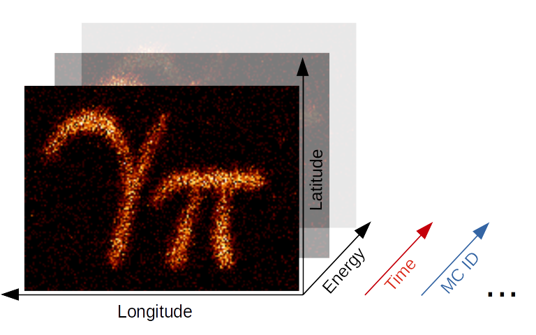
The maps submodule contains classes for representing pixilised data on the sky with an arbitrary number of non-spatial dimensions such as energy, time, event class or any possible user-defined dimension (illustrated in the image above). The main Map data structure features a uniform API for WCS as well as HEALPix based images. The API also generalizes simple image based operations such as smoothing, interpolation and reprojection to the arbitrary extra dimensions and makes working with (2 + N)-dimensional hypercubes as easy as working with a simple 2D image. Further information is also provided on the maps docs page.

In the following introduction we will learn all the basics of working with WCS based maps. HEALPix based maps will be covered in a future tutorial. Make sure you have worked through the Gammapy overview, because a solid knowledge about working with SkyCoord and Quantity objects as well as Numpy is required for this tutorial.

This notebook is rather lengthy, but getting to know the Map data structure in detail is essential for working with Gammapy and will allow you to fulfill complex analysis tasks with very few and simple code in future!

Setup

import os

# %matplotlib inline
import numpy as np
from astropy import units as u
from astropy.convolution import convolve
from astropy.coordinates import SkyCoord
from astropy.io import fits
from astropy.table import Table
from astropy.time import Time
import matplotlib.pyplot as plt
from IPython.display import display
from gammapy.data import EventList
from gammapy.maps import (
    LabelMapAxis,
    Map,
    MapAxes,
    MapAxis,
    TimeMapAxis,
    WcsGeom,
    WcsNDMap,
)

Check setup

from gammapy.utils.check import check_tutorials_setup

check_tutorials_setup()

System:

        python_executable      : /home/runner/work/gammapy-docs/gammapy-docs/gammapy/.tox/build_docs/bin/python
        python_version         : 3.9.20
        machine                : x86_64
        system                 : Linux


Gammapy package:

        version                : 2.0.dev155+g9309a089d
        path                   : /home/runner/work/gammapy-docs/gammapy-docs/gammapy/.tox/build_docs/lib/python3.9/site-packages/gammapy


Other packages:

        numpy                  : 1.26.4
        scipy                  : 1.13.1
        astropy                : 5.2.2
        regions                : 0.8
        click                  : 8.1.7
        yaml                   : 6.0.2
        IPython                : 8.18.1
        jupyterlab             : not installed
        matplotlib             : 3.9.4
        pandas                 : not installed
        healpy                 : 1.17.3
        iminuit                : 2.30.1
        sherpa                 : 4.16.1
        naima                  : 0.10.0
        emcee                  : 3.1.6
        corner                 : 2.2.3
        ray                    : 2.40.0


Gammapy environment variables:

        GAMMAPY_DATA           : /home/runner/work/gammapy-docs/gammapy-docs/gammapy-datasets/dev

Creating WCS Maps

Using Factory Methods

Maps are most easily created using the create factory method:

m_allsky = Map.create()

Calling create without any further arguments creates by default an allsky WCS map using a CAR projection, ICRS coordinates and a pixel size of 1 deg. This can be easily checked by printing the geom attribute of the map:

print(m_allsky.geom)

WcsGeom

        axes       : ['lon', 'lat']
        shape      : (3600, 1800)
        ndim       : 2
        frame      : icrs
        projection : CAR
        center     : 0.0 deg, 0.0 deg
        width      : 360.0 deg x 180.0 deg
        wcs ref    : 0.0 deg, 0.0 deg

The geom attribute is a Geom object, that defines the basic geometry of the map, such as size of the pixels, width and height of the image, coordinate system etc., but we will learn more about this object later.

Besides the .geom attribute the map has also a .data attribute, which is just a plain ~numpy.ndarray and stores the data associated with this map:

print(m_allsky.data)

[[0. 0. 0. ... 0. 0. 0.]
 [0. 0. 0. ... 0. 0. 0.]
 [0. 0. 0. ... 0. 0. 0.]
 ...
 [0. 0. 0. ... 0. 0. 0.]
 [0. 0. 0. ... 0. 0. 0.]
 [0. 0. 0. ... 0. 0. 0.]]

By default maps are filled with zeros.

The map_type argument can be used to control the pixelization scheme (WCS or HPX).

position = SkyCoord(0.0, 5.0, frame="galactic", unit="deg")

# Create a WCS Map
m_wcs = Map.create(binsz=0.1, map_type="wcs", skydir=position, width=10.0)

# Create a HPX Map
m_hpx = Map.create(binsz=0.1, map_type="hpx", skydir=position, width=10.0)

Here is an example that creates a WCS map centered on the Galactic center and now uses Galactic coordinates:

skydir = SkyCoord(0, 0, frame="galactic", unit="deg")
m_gc = Map.create(
    binsz=0.02, width=(10, 5), skydir=skydir, frame="galactic", proj="TAN"
)
print(m_gc.geom)

WcsGeom

        axes       : ['lon', 'lat']
        shape      : (500, 250)
        ndim       : 2
        frame      : galactic
        projection : TAN
        center     : 0.0 deg, 0.0 deg
        width      : 10.0 deg x 5.0 deg
        wcs ref    : 0.0 deg, 0.0 deg

In addition we have defined a TAN projection, a pixel size of 0.02 deg and a width of the map of 10 deg x 5 deg. The width argument also takes scalar value instead of a tuple, which is interpreted as both the width and height of the map, so that a quadratic map is created.

Creating from a Map Geometry

As we have seen in the first examples, the Map object couples the data (stored as a ndarray) with a Geom object. The ~Geom object can be seen as a generalization of an astropy.wcs.WCS object, providing the information on how the data maps to physical coordinate systems. In some cases e.g. when creating many maps with the same WCS geometry it can be advantageous to first create the map geometry independent of the map object it-self:

wcs_geom = WcsGeom.create(binsz=0.02, width=(10, 5), skydir=(0, 0), frame="galactic")

And then create the map objects from the wcs_geom geometry specification:

maps = {}

for name in ["counts", "background"]:
    maps[name] = Map.from_geom(wcs_geom)

The Geom object also has a few helpful methods. E.g. we can check whether a given position on the sky is contained in the map geometry:

# define the position of the Galactic center and anti-center
positions = SkyCoord([0, 180], [0, 0], frame="galactic", unit="deg")
wcs_geom.contains(positions)

array([ True, False])

Or get the image center of the map:

print(wcs_geom.center_skydir)

<SkyCoord (Galactic): (l, b) in deg
    (0., 0.)>

Or we can also retrieve the solid angle per pixel of the map:

print(wcs_geom.solid_angle())

[[1.21731921e-07 1.21731921e-07 1.21731921e-07 ... 1.21731921e-07
  1.21731921e-07 1.21731921e-07]
 [1.21733761e-07 1.21733761e-07 1.21733761e-07 ... 1.21733761e-07
  1.21733761e-07 1.21733761e-07]
 [1.21735587e-07 1.21735587e-07 1.21735587e-07 ... 1.21735587e-07
  1.21735587e-07 1.21735587e-07]
 ...
 [1.21735587e-07 1.21735587e-07 1.21735587e-07 ... 1.21735587e-07
  1.21735587e-07 1.21735587e-07]
 [1.21733761e-07 1.21733761e-07 1.21733761e-07 ... 1.21733761e-07
  1.21733761e-07 1.21733761e-07]
 [1.21731921e-07 1.21731921e-07 1.21731921e-07 ... 1.21731921e-07
  1.21731921e-07 1.21731921e-07]] sr

Adding Non-Spatial Axes

In many analysis scenarios we would like to add extra dimension to the maps to study e.g. energy or time dependency of the data. Those non-spatial dimensions are handled with the MapAxis object. Let us first define an energy axis, with 4 bins:

energy_axis = MapAxis.from_bounds(
    1, 100, nbin=4, unit="TeV", name="energy", interp="log"
)
print(energy_axis)

MapAxis

        name       : energy
        unit       : 'TeV'
        nbins      : 4
        node type  : edges
        edges min  : 1.0e+00 TeV
        edges max  : 1.0e+02 TeV
        interp     : log

Where interp='log' specifies that a logarithmic spacing is used between the bins, equivalent to np.logspace(0, 2, 4). This MapAxis object we can now pass to create() using the axes= argument:

m_cube = Map.create(binsz=0.02, width=(10, 5), frame="galactic", axes=[energy_axis])
print(m_cube.geom)

WcsGeom

        axes       : ['lon', 'lat', 'energy']
        shape      : (500, 250, 4)
        ndim       : 3
        frame      : galactic
        projection : CAR
        center     : 0.0 deg, 0.0 deg
        width      : 10.0 deg x 5.0 deg
        wcs ref    : 0.0 deg, 0.0 deg

Now we see that besides lon and lat the map has an additional axes named energy with 4 bins. The total dimension of the map is now ndim=3.

We can also add further axes by passing a list of MapAxis objects. To demonstrate this we create a time axis with linearly spaced bins and pass both axes to Map.create():

time_axis = MapAxis.from_bounds(0, 24, nbin=24, unit="hour", name="time", interp="lin")

m_4d = Map.create(
    binsz=0.02, width=(10, 5), frame="galactic", axes=[energy_axis, time_axis]
)
print(m_4d.geom)

WcsGeom

        axes       : ['lon', 'lat', 'energy', 'time']
        shape      : (500, 250, 4, 24)
        ndim       : 4
        frame      : galactic
        projection : CAR
        center     : 0.0 deg, 0.0 deg
        width      : 10.0 deg x 5.0 deg
        wcs ref    : 0.0 deg, 0.0 deg

The MapAxis object internally stores the coordinates or “position values” associated with every map axis bin or “node”. We distinguish between two node types: "edges" and "center". The node type "edges"(which is also the default) specifies that the data associated with this axis is integrated between the edges of the bin (e.g. counts data). The node type "center" specifies that the data is given at the center of the bin (e.g. exposure or differential fluxes).

The edges of the bins can be checked with edges attribute:

print(energy_axis.edges)

[  1.           3.16227766  10.          31.6227766  100.        ] TeV

The numbers are given in the units we specified above, which can be checked again with:

print(energy_axis.unit)

TeV

The centers of the axis bins can be checked with the center attribute:

print(energy_axis.center)

[ 1.77827941  5.62341325 17.7827941  56.23413252] TeV

Adding Non-contiguous axes

Non-spatial map axes can also be handled through two other objects known as the TimeMapAxis and the LabelMapAxis.

TimeMapAxis

The TimeMapAxis object provides an axis for non-adjacent time intervals.

time_map_axis = TimeMapAxis(
    edges_min=[1, 5, 10, 15] * u.day,
    edges_max=[2, 7, 13, 18] * u.day,
    reference_time=Time("2020-03-19"),
)

print(time_map_axis)

TimeMapAxis
-----------

  name           : time
  nbins          : 4
  reference time : 2020-03-19 00:00:00.000
  scale          : utc
  time min.      : 2020-03-20 00:00:00.000
  time max.      : 2020-04-06 00:00:00.000
  total time     : 216.0 h

This time_map_axis can then be utilised in a similar way to the previous implementation to create a Map.

map_4d = Map.create(
    binsz=0.02, width=(10, 5), frame="galactic", axes=[energy_axis, time_map_axis]
)
print(map_4d.geom)

WcsGeom

        axes       : ['lon', 'lat', 'energy', 'time']
        shape      : (500, 250, 4, 4)
        ndim       : 4
        frame      : galactic
        projection : CAR
        center     : 0.0 deg, 0.0 deg
        width      : 10.0 deg x 5.0 deg
        wcs ref    : 0.0 deg, 0.0 deg

It is possible to utilise the slice attrribute to create new a TimeMapAxis. Here we are slicing between the first and third axis to extract the subsection of the axis between indice 0 and 2.

print(time_map_axis.slice([0, 2]))

TimeMapAxis
-----------

  name           : time
  nbins          : 2
  reference time : 2020-03-19 00:00:00.000
  scale          : utc
  time min.      : 2020-03-20 00:00:00.000
  time max.      : 2020-04-01 00:00:00.000
  total time     : 96.0 h

It is also possible to squash the axis, which squashes the existing axis into one bin. This creates a new axis between the extreme edges of the initial axis.

print(time_map_axis.squash())

TimeMapAxis
-----------

  name           : time
  nbins          : 1
  reference time : 2020-03-19 00:00:00.000
  scale          : utc
  time min.      : 2020-03-20 00:00:00.000
  time max.      : 2020-04-06 00:00:00.000
  total time     : 408.0 h

The is_contiguous method returns a boolean which indicates whether the TimeMapAxis is contiguous or not.

print(time_map_axis.is_contiguous)

False

As we have a non-contiguous axis we can print the array of bin edges for both the minimum axis edges (edges_min) and the maximum axis edges (edges_max).

print(time_map_axis.edges_min)

print(time_map_axis.edges_max)

[ 1.  5. 10. 15.] d
[ 2.  7. 13. 18.] d

Next, we use the to_contiguous functionality to create a contiguous axis and expose edges. This method returns a Quantity with respect to the reference time.

time_map_axis_contiguous = time_map_axis.to_contiguous()

print(time_map_axis_contiguous.is_contiguous)

print(time_map_axis_contiguous.edges)

True
[ 1.  2.  5.  7. 10. 13. 15. 18.] d

The time_edges will return the Time object directly

print(time_map_axis_contiguous.time_edges)

['2020-03-20 00:00:00.000' '2020-03-21 00:00:00.000'
 '2020-03-24 00:00:00.000' '2020-03-26 00:00:00.000'
 '2020-03-29 00:00:00.000' '2020-04-01 00:00:00.000'
 '2020-04-03 00:00:00.000' '2020-04-06 00:00:00.000']

TimeMapAxis also has both functionalities of coord_to_pix and coord_to_idx. The coord_to_idx attribute will give the index of the time specified, similarly for coord_to_pix which returns the pixel. A linear interpolation is assumed.

Start by choosing a time which we know is within the TimeMapAxis and see the results.

time = Time(time_map_axis.time_max.mjd[0], format="mjd")

print(time_map_axis.coord_to_pix(time))

print(time_map_axis.coord_to_idx(time))

[0.5]
0

This functionality can also be used with an array of Time values.

times = Time(time_map_axis.time_max.mjd, format="mjd")

print(time_map_axis.coord_to_pix(times))

print(time_map_axis.coord_to_idx(times))

[0.5 1.5 2.5 3.5]
[0 1 2 3]

Note here we take a Time which is outside the edges. A linear interpolation is assumed for both methods, therefore for a time outside the time_map_axis there is no extrapolation and -1 is returned.

Note: due to this, the coord_to_pix method will return nan and the coord_to_idx method returns -1.

print(time_map_axis.coord_to_pix(Time(time.mjd + 1, format="mjd")))

print(time_map_axis.coord_to_idx(Time(time.mjd + 1, format="mjd")))

[nan]
-1

LabelMapAxis

The LabelMapAxis object allows for handling of labels for map axes. It provides an axis for non-numeric entries.

label_axis = LabelMapAxis(
    labels=["dataset-1", "dataset-2", "dataset-3"], name="dataset"
)

print(label_axis)

LabelMapAxis
------------

  name       : dataset
  nbins      : 3
  node type  : label
  labels     : ['dataset-1', 'dataset-2', 'dataset-3']

The labels can be checked using the center attribute:

print(label_axis.center)

['dataset-1' 'dataset-2' 'dataset-3']

To obtain the position of the label, one can utilise the coord_to_pix attribute

print(label_axis.coord_to_pix(["dataset-3"]))

[2.]

To adapt and create new axes the following attributes can be utilised: concatenate, slice and squash.

Combining two different LabelMapAxis is done in the following way:

label_axis2 = LabelMapAxis(labels=["dataset-a", "dataset-b"], name="dataset")

print(label_axis.concatenate(label_axis2))

LabelMapAxis
------------

  name       : dataset
  nbins      : 5
  node type  : label
  labels     : ['dataset-1', 'dataset-2', 'dataset-3', 'dataset-a', 'dataset-b']

A new LabelMapAxis can be created by slicing an already existing one. Here we are slicing between the second and third bins to extract the subsection.

print(label_axis.slice([1, 2]))

LabelMapAxis
------------

  name       : dataset
  nbins      : 2
  node type  : label
  labels     : ['dataset-2', 'dataset-3']

A new axis object can be created by squashing the axis into a single bin.

print(label_axis.squash())

LabelMapAxis
------------

  name       : dataset
  nbins      : 1
  node type  : label
  labels     : ['dataset-1...dataset-3']

Mixing the three previous axis types (MapAxis, TimeMapAxis and LabelMapAxis) would be done like so:

axes = MapAxes(axes=[energy_axis, time_map_axis, label_axis])
hdu = axes.to_table_hdu(format="gadf")
table = Table.read(hdu)
display(table)

CHANNEL       ENERGY             E_MIN        ... TIME_MIN TIME_MAX  DATASET
               TeV                TeV         ...    d        d
------- ------------------ ------------------ ... -------- -------- ---------
      0  1.778279410038923                1.0 ...      1.0      2.0 dataset-1
      1  1.778279410038923                1.0 ...      1.0      2.0 dataset-2
      2  1.778279410038923                1.0 ...      1.0      2.0 dataset-3
      3  5.623413251903492 3.1622776601683795 ...      1.0      2.0 dataset-1
      4  5.623413251903492 3.1622776601683795 ...      1.0      2.0 dataset-2
      5  5.623413251903492 3.1622776601683795 ...      1.0      2.0 dataset-3
      6  17.78279410038923 10.000000000000002 ...      1.0      2.0 dataset-1
      7  17.78279410038923 10.000000000000002 ...      1.0      2.0 dataset-2
      8  17.78279410038923 10.000000000000002 ...      1.0      2.0 dataset-3
      9 56.234132519034915  31.62277660168379 ...      1.0      2.0 dataset-1
    ...                ...                ... ...      ...      ...       ...
     38  1.778279410038923                1.0 ...     15.0     18.0 dataset-3
     39  5.623413251903492 3.1622776601683795 ...     15.0     18.0 dataset-1
     40  5.623413251903492 3.1622776601683795 ...     15.0     18.0 dataset-2
     41  5.623413251903492 3.1622776601683795 ...     15.0     18.0 dataset-3
     42  17.78279410038923 10.000000000000002 ...     15.0     18.0 dataset-1
     43  17.78279410038923 10.000000000000002 ...     15.0     18.0 dataset-2
     44  17.78279410038923 10.000000000000002 ...     15.0     18.0 dataset-3
     45 56.234132519034915  31.62277660168379 ...     15.0     18.0 dataset-1
     46 56.234132519034915  31.62277660168379 ...     15.0     18.0 dataset-2
     47 56.234132519034915  31.62277660168379 ...     15.0     18.0 dataset-3
Length = 48 rows

Reading and Writing

Gammapy Map objects are serialized using the Flexible Image Transport Format (FITS). Depending on the pixelization scheme (HEALPix or WCS) and presence of non-spatial dimensions the actual convention to write the FITS file is different. By default Gammapy uses a generic convention named "gadf", which will support WCS and HEALPix formats as well as an arbitrary number of non-spatial axes. The convention is documented in detail on the Gamma Astro Data Formats page.

Other conventions required by specific software (e.g. the Fermi Science Tools) are supported as well. At the moment those are the following

• "fgst-ccube": Fermi counts cube format.

• "fgst-ltcube": Fermi livetime cube format.

• "fgst-bexpcube": Fermi exposure cube format

• "fgst-template": Fermi Galactic diffuse and source template format.

• "fgst-srcmap" and "fgst-srcmap-sparse": Fermi source map and sparse source map format.

The conventions listed above only support an additional energy axis.

Reading Maps

Reading FITS files is mainly exposed via the read() method. Let us take a look at a first example:

filename = "$GAMMAPY_DATA/fermi-3fhl-gc/fermi-3fhl-gc-counts.fits.gz"
m_3fhl_gc = Map.read(filename)
print(m_3fhl_gc)

WcsNDMap

        geom  : WcsGeom
        axes  : ['lon', 'lat']
        shape : (400, 200)
        ndim  : 2
        unit  :
        dtype : >i8

If map_type argument is not given when calling read a map object will be instantiated with the pixelization of the input HDU.

By default Map.read() will try to find the first valid data hdu in the filename and read the data from there. If multiple HDUs are present in the FITS file, the desired one can be chosen with the additional hdu= argument:

m_3fhl_gc = Map.read(filename, hdu="PRIMARY")
print(m_3fhl_gc)

WcsNDMap

        geom  : WcsGeom
        axes  : ['lon', 'lat']
        shape : (400, 200)
        ndim  : 2
        unit  :
        dtype : >i8

In rare cases e.g. when the FITS file is not valid or meta data is missing from the header it can be necessary to modify the header of a certain HDU before creating the Map object. In this case we can use astropy.io.fits directly to read the FITS file:

filename = os.environ["GAMMAPY_DATA"] + "/fermi-3fhl-gc/fermi-3fhl-gc-exposure.fits.gz"
hdulist = fits.open(filename)
print(hdulist.info())

Filename: /home/runner/work/gammapy-docs/gammapy-docs/gammapy-datasets/dev/fermi-3fhl-gc/fermi-3fhl-gc-exposure.fits.gz
No.    Name      Ver    Type      Cards   Dimensions   Format
  0  PRIMARY       1 PrimaryHDU      23   (400, 200)   float32
None

And then modify the header keyword and use Map.from_hdulist() to create the Map object after:

hdulist["PRIMARY"].header["BUNIT"] = "cm2 s"
print(Map.from_hdulist(hdulist=hdulist))

WcsNDMap

        geom  : WcsGeom
        axes  : ['lon', 'lat']
        shape : (400, 200)
        ndim  : 2
        unit  : cm2 s
        dtype : >f4

Writing Maps

Writing FITS files on disk via the Map.write() method. Here is a first example:

m_cube.write("example_cube.fits", overwrite=True)

By default Gammapy does not overwrite files. In this example we set overwrite=True in case the cell gets executed multiple times. Now we can read back the cube from disk using Map.read():

m_cube = Map.read("example_cube.fits")
print(m_cube)

WcsNDMap

        geom  : WcsGeom
        axes  : ['lon', 'lat', 'energy']
        shape : (500, 250, 4)
        ndim  : 3
        unit  :
        dtype : >f4

We can also choose a different FITS convention to write the example cube in a format compatible to the Fermi Galactic diffuse background model:

m_cube.write("example_cube_fgst.fits", format="fgst-template", overwrite=True)

To understand a little bit better the generic gadf convention we use Map.to_hdulist() to generate a list of FITS HDUs first:

hdulist = m_4d.to_hdulist(format="gadf")
print(hdulist.info())

Filename: (No file associated with this HDUList)
No.    Name      Ver    Type      Cards   Dimensions   Format
  0  PRIMARY       1 PrimaryHDU      30   (500, 250, 4, 24)   float32
  1  PRIMARY_BANDS    1 BinTableHDU     33   96R x 7C   ['K', 'D', 'D', 'D', 'D', 'D', 'D']
None

As we can see the HDUList object contains to HDUs. The first one named PRIMARY contains the data array with shape corresponding to our data and the WCS information stored in the header:

print(hdulist["PRIMARY"].header)

SIMPLE  =                    T / conforms to FITS standard                      BITPIX  =                  -32 / array data type                                NAXIS   =                    4 / number of array dimensions                     NAXIS1  =                  500                                                  NAXIS2  =                  250                                                  NAXIS3  =                    4                                                  NAXIS4  =                   24                                                  EXTEND  =                    T                                                  WCSAXES =                    2 / Number of coordinate axes                      CRPIX1  =                250.5 / Pixel coordinate of reference point            CRPIX2  =                125.5 / Pixel coordinate of reference point            CDELT1  =                -0.02 / [deg] Coordinate increment at reference point  CDELT2  =                 0.02 / [deg] Coordinate increment at reference point  CUNIT1  = 'deg'                / Units of coordinate increment and value        CUNIT2  = 'deg'                / Units of coordinate increment and value        CTYPE1  = 'GLON-CAR'           / galactic longitude, plate caree projection     CTYPE2  = 'GLAT-CAR'           / galactic latitude, plate caree projection      CRVAL1  =                  0.0 / [deg] Coordinate value at reference point      CRVAL2  =                  0.0 / [deg] Coordinate value at reference point      LONPOLE =                  0.0 / [deg] Native longitude of celestial pole       LATPOLE =                 90.0 / [deg] Native latitude of celestial pole        MJDREF  =                  0.0 / [d] MJD of fiducial time                       AXCOLS1 = 'E_MIN,E_MAX'                                                         INTERP1 = 'log     '                                                            AXCOLS2 = 'TIME_MIN,TIME_MAX'                                                   INTERP2 = 'lin     '                                                            WCSSHAPE= '(500,250,4,24)'                                                      BANDSHDU= 'PRIMARY_BANDS'                                                       META    = '{}      '                                                            BUNIT   = ''                                                                    END

The second HDU is a BinTableHDU named PRIMARY_BANDS contains the information on the non-spatial axes such as name, order, unit, min, max and center values of the axis bins. We use an astropy.table.Table to show the information:

print(Table.read(hdulist["PRIMARY_BANDS"]))

CHANNEL       ENERGY             E_MIN        ... TIME TIME_MIN TIME_MAX
               TeV                TeV         ...  h      h        h
------- ------------------ ------------------ ... ---- -------- --------
      0  1.778279410038923                1.0 ...  0.5      0.0      1.0
      1  5.623413251903492 3.1622776601683795 ...  0.5      0.0      1.0
      2  17.78279410038923 10.000000000000002 ...  0.5      0.0      1.0
      3 56.234132519034915  31.62277660168379 ...  0.5      0.0      1.0
      4  1.778279410038923                1.0 ...  1.5      1.0      2.0
      5  5.623413251903492 3.1622776601683795 ...  1.5      1.0      2.0
      6  17.78279410038923 10.000000000000002 ...  1.5      1.0      2.0
      7 56.234132519034915  31.62277660168379 ...  1.5      1.0      2.0
      8  1.778279410038923                1.0 ...  2.5      2.0      3.0
      9  5.623413251903492 3.1622776601683795 ...  2.5      2.0      3.0
    ...                ...                ... ...  ...      ...      ...
     86  17.78279410038923 10.000000000000002 ... 21.5     21.0     22.0
     87 56.234132519034915  31.62277660168379 ... 21.5     21.0     22.0
     88  1.778279410038923                1.0 ... 22.5     22.0     23.0
     89  5.623413251903492 3.1622776601683795 ... 22.5     22.0     23.0
     90  17.78279410038923 10.000000000000002 ... 22.5     22.0     23.0
     91 56.234132519034915  31.62277660168379 ... 22.5     22.0     23.0
     92  1.778279410038923                1.0 ... 23.5     23.0     24.0
     93  5.623413251903492 3.1622776601683795 ... 23.5     23.0     24.0
     94  17.78279410038923 10.000000000000002 ... 23.5     23.0     24.0
     95 56.234132519034915  31.62277660168379 ... 23.5     23.0     24.0
Length = 96 rows

Maps can be serialized to a sparse data format by calling write with sparse=True. This will write all non-zero pixels in the map to a data table appropriate to the pixelization scheme.

m = Map.create(binsz=0.1, map_type="wcs", width=10.0)
m.write("file.fits", hdu="IMAGE", sparse=True, overwrite=True)
m = Map.read("file.fits", hdu="IMAGE", map_type="wcs")

Accessing Data

How to get data values

All map objects have a set of accessor methods, which can be used to access or update the contents of the map irrespective of its underlying representation. Those accessor methods accept as their first argument a coordinate tuple containing scalars, list, or numpy.ndarray with one tuple element for each dimension. Some methods additionally accept a dict or MapCoord argument, of which both allow to assign coordinates by axis name.

Let us first begin with the get_by_idx() method, that accepts a tuple of indices. The order of the indices corresponds to the axis order of the map:

print(m_gc.get_by_idx((50, 30)))

[0.]

Important: Gammapy uses a reversed index order in the map API with the longitude axes first. To achieve the same by directly indexing into the numpy array we have to call:

print(m_gc.data[([30], [50])])

[0.]

To check the order of the axes you can always print the .geom` attribute:

print(m_gc.geom)

WcsGeom

        axes       : ['lon', 'lat']
        shape      : (500, 250)
        ndim       : 2
        frame      : galactic
        projection : TAN
        center     : 0.0 deg, 0.0 deg
        width      : 10.0 deg x 5.0 deg
        wcs ref    : 0.0 deg, 0.0 deg

To access values directly by sky coordinates we can use the get_by_coord() method. This time we pass in a dict, specifying the axes names corresponding to the given coordinates:

print(m_gc.get_by_coord({"lon": [0, 180], "lat": [0, 0]}))

[ 0. nan]

The units of the coordinates are assumed to be in degrees in the coordinate system used by the map. If the coordinates do not correspond to the exact pixel center, the value of the nearest pixel center will be returned. For positions outside the map geometry np.nan is returned.

The coordinate or idx arrays follow normal Numpy broadcasting rules. So the following works as expected:

lons = np.linspace(-4, 4, 10)
print(m_gc.get_by_coord({"lon": lons, "lat": 0}))

[0. 0. 0. 0. 0. 0. 0. 0. 0. 0.]

Or as an even more advanced example, we can provide lats as column vector and broadcasting to a 2D result array will be applied:

lons = np.linspace(-4, 4, 8)
lats = np.linspace(-4, 4, 8).reshape(-1, 1)
print(m_gc.get_by_coord({"lon": lons, "lat": lats}))

[[nan nan nan nan nan nan nan nan]
 [nan nan nan nan nan nan nan nan]
 [ 0.  0.  0.  0.  0.  0.  0.  0.]
 [ 0.  0.  0.  0.  0.  0.  0.  0.]
 [ 0.  0.  0.  0.  0.  0.  0.  0.]
 [ 0.  0.  0.  0.  0.  0.  0.  0.]
 [nan nan nan nan nan nan nan nan]
 [nan nan nan nan nan nan nan nan]]

Indexing and Slicing Sub-Maps

When you have worked with Numpy arrays in the past you are probably familiar with the concept of indexing and slicing into data arrays. To support slicing of non-spatial axes of Map objects, the Map object has a slice_by_idx() method, which allows to extract sub-maps from a larger map.

The following example demonstrates how to get the map at the energy bin number 3:

m_sub = m_cube.slice_by_idx({"energy": 3})
print(m_sub)

WcsNDMap

        geom  : WcsGeom
        axes  : ['lon', 'lat']
        shape : (500, 250)
        ndim  : 2
        unit  :
        dtype : >f4

Note that the returned object is again a Map with updated axes information. In this case, because we extracted only a single image, the energy axes is dropped from the map.

To extract a sub-cube with a sliced energy axes we can use a normal slice() object:

m_sub = m_cube.slice_by_idx({"energy": slice(1, 3)})
print(m_sub)

WcsNDMap

        geom  : WcsGeom
        axes  : ['lon', 'lat', 'energy']
        shape : (500, 250, 2)
        ndim  : 3
        unit  :
        dtype : >f4

Note that the returned object is also a Map object, but this time with updated energy axis specification.

Slicing of multiple dimensions is supported by adding further entries to the dict passed to slice_by_idx()

m_sub = m_4d.slice_by_idx({"energy": slice(1, 3), "time": slice(4, 10)})
print(m_sub)

WcsNDMap

        geom  : WcsGeom
        axes  : ['lon', 'lat', 'energy', 'time']
        shape : (500, 250, 2, 6)
        ndim  : 4
        unit  :
        dtype : float32

For convenience there is also a get_image_by_coord() method which allows to access image planes at given non-spatial physical coordinates. This method also supports Quantity objects:

image = m_4d.get_image_by_coord({"energy": 4 * u.TeV, "time": 5 * u.h})
print(image.geom)

WcsGeom

        axes       : ['lon', 'lat']
        shape      : (500, 250)
        ndim       : 2
        frame      : galactic
        projection : CAR
        center     : 0.0 deg, 0.0 deg
        width      : 10.0 deg x 5.0 deg
        wcs ref    : 0.0 deg, 0.0 deg

Iterating by image

For maps with non-spatial dimensions the iter_by_image_data method can be used to loop over image slices. The image plane index idx is returned in data order, so that the data array can be indexed directly. Here is an example for an in-place convolution of an image using convolve to interpolate NaN values:

axis1 = MapAxis([1, 10, 100], interp="log", name="energy")
axis2 = MapAxis([1, 2, 3], interp="lin", name="time")
m = Map.create(width=(5, 3), axes=[axis1, axis2], binsz=0.1)
m.data[:, :, 15:18, 20:25] = np.nan

for img, idx in m.iter_by_image_data():
    kernel = np.ones((5, 5))
    m.data[idx] = convolve(img, kernel)

assert not np.isnan(m.data).any()

Modifying Data

How to set data values

To modify and set map data values the Map object features as well a set_by_idx() method:

m_cube.set_by_idx(idx=(10, 20, 3), vals=42)

here we check that data have been updated:

print(m_cube.get_by_idx((10, 20, 3)))

[42.]

Of course there is also a set_by_coord() method, which allows to set map data values in physical coordinates.

m_cube.set_by_coord({"lon": 0, "lat": 0, "energy": 2 * u.TeV}, vals=42)

Again the lon and lat values are assumed to be given in degrees in the coordinate system used by the map. For the energy axis, the unit is the one specified on the axis (use m_cube.geom.axes[0].unit to check if needed…).

All .xxx_by_coord() methods accept SkyCoord objects as well. In this case we have to use the "skycoord" keyword instead of "lon" and "lat":

skycoords = SkyCoord([1.2, 3.4], [-0.5, 1.1], frame="galactic", unit="deg")
m_cube.set_by_coord({"skycoord": skycoords, "energy": 2 * u.TeV}, vals=42)

Filling maps from event lists

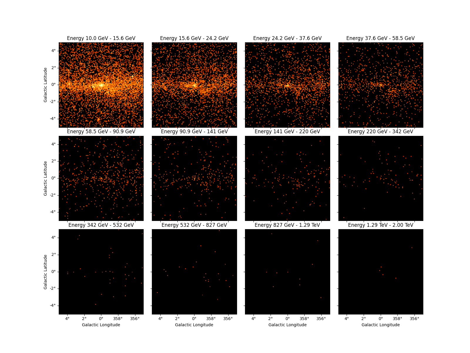
This example shows how to fill a counts cube from an event list:

energy_axis = MapAxis.from_bounds(
    10.0, 2e3, 12, interp="log", name="energy", unit="GeV"
)
counts_3d = WcsNDMap.create(
    binsz=0.1, width=10.0, skydir=(0, 0), frame="galactic", axes=[energy_axis]
)

events = EventList.read("$GAMMAPY_DATA/fermi-3fhl-gc/fermi-3fhl-gc-events.fits.gz")

counts_3d.fill_by_coord({"skycoord": events.radec, "energy": events.energy})
counts_3d.write("ccube.fits", format="fgst-ccube", overwrite=True)

Alternatively you can use the fill_events method:

counts_3d = WcsNDMap.create(
    binsz=0.1, width=10.0, skydir=(0, 0), frame="galactic", axes=[energy_axis]
)

counts_3d.fill_events(events)

If you have a given map already, and want to make a counts image with the same geometry (not using the pixel data from the original map), you can also use the fill_events method.

events = EventList.read("$GAMMAPY_DATA/fermi-3fhl-gc/fermi-3fhl-gc-events.fits.gz")
reference_map = Map.read("$GAMMAPY_DATA/fermi-3fhl-gc/fermi-3fhl-gc-counts.fits.gz")
counts = Map.from_geom(reference_map.geom)
counts.fill_events(events)

It works for IACT and Fermi-LAT events, for WCS or HEALPix map geometries, and also for extra axes. Especially energy axes are automatically handled correctly.

Filling maps from interpolation

Maps support interpolation via the interp_by_coord and interp_by_pix methods. Currently, the following interpolation methods are supported:

• "nearest" : Return value of nearest pixel (no interpolation).

• "linear" : Interpolation with first order polynomial. This is the only interpolation method that is supported for all map types.

• quadratic : Interpolation with second order polynomial.

• cubic : Interpolation with third order polynomial.

Note that "quadratic" and "cubic" interpolation are currently only supported for WCS-based maps with regular geometry (e.g. 2D or ND with the same geometry in every image plane). "linear" and higher order interpolation by pixel coordinates is only supported for WCS-based maps.

In the following example we create a new map and fill it by interpolating another map:

# read map
filename = "$GAMMAPY_DATA/fermi-3fhl-gc/gll_iem_v06_gc.fits.gz"
m_iem_gc = Map.read(filename)

# create new geometry
skydir = SkyCoord(266.4, -28.9, frame="icrs", unit="deg")
wcs_geom_cel = WcsGeom.create(skydir=skydir, binsz=0.1, frame="icrs", width=(8, 4))

# create new empty map from geometry
m_iem_10GeV = Map.from_geom(wcs_geom_cel)
coords = m_iem_10GeV.geom.get_coord()

# fill new map using interpolation
m_iem_10GeV.data = m_iem_gc.interp_by_coord(
    {"skycoord": coords.skycoord, "energy_true": 10 * u.GeV},
    method="linear",
    fill_value=np.nan,
)

Interpolating onto a different geometry

For 3d geometries this operation can be performed directly using the interp_to_geom() method. This is very useful, ex: while using map arithmetic.

# create new geometry
energy_axis = MapAxis.from_bounds(
    10.0, 2e3, 6, interp="log", name="energy_true", unit="GeV"
)
skydir = SkyCoord(266.4, -28.9, frame="icrs", unit="deg")
wcs_geom_3d = WcsGeom.create(
    skydir=skydir, binsz=0.1, frame="icrs", width=(8, 4), axes=[energy_axis]
)

# create the interpolated map
m_iem_interp = m_iem_gc.interp_to_geom(
    wcs_geom_3d, preserve_counts=False, method="linear", fill_value=np.nan
)
print(m_iem_interp)

WcsNDMap

        geom  : WcsGeom
        axes  : ['lon', 'lat', 'energy_true']
        shape : (80, 40, 6)
        ndim  : 3
        unit  : 1 / (cm2 MeV s sr)
        dtype : float64

Note that preserve_counts= option should be true if the map is an integral quantity (e.g. counts) and false if the map is a differential quantity (e.g. intensity).

Maps operations

Basic operators

One can perform simple arithmetic on maps using the +, -, *, / operators, this works only for maps with the same geometry:

iem_plus_iem = m_iem_10GeV + m_iem_10GeV

iem_minus_iem = m_iem_10GeV - m_iem_10GeV

These operations can be applied between a Map and a scalar in that specific order:

iem_times_two = m_iem_10GeV * 2
# iem_times_two = 2 * m_iem_10GeV # this won't work

The logic operators can also be applied on maps (the result is a map of boolean type):

is_null = iem_minus_iem == 0
print(is_null)

WcsNDMap

        geom  : WcsGeom
        axes  : ['lon', 'lat']
        shape : (80, 40)
        ndim  : 2
        unit  :
        dtype : bool

Here we check that the result is True for all the well-defined pixels (not NaN):

print(np.all(is_null.data[~np.isnan(iem_minus_iem)]))

True

Cutouts

The WCSNDMap objects features a cutout() method, which allows you to cut out a smaller part of a larger map. This can be useful, e.g. when working with all-sky diffuse maps. Here is an example:

position = SkyCoord(0, 0, frame="galactic", unit="deg")
m_iem_cutout = m_iem_gc.cutout(position=position, width=(4 * u.deg, 2 * u.deg))

The returned object is again a Map object with updated WCS information and data size. As one can see the cutout is automatically applied to all the non-spatial axes as well. The cutout width is given in the order of (lon, lat) and can be specified with units that will be handled correctly.

Visualizing and Plotting

All map objects provide a plot method for generating a visualization of a map. This method returns figure, axes, and image objects that can be used to further tweak/customize the image. The plot method should be used with 2D maps, while 3D maps can be displayed with the plot_interactive() or plot_grid() methods.

Image Plotting

For debugging and inspecting the map data it is useful to plot or visualize the images planes contained in the map.

filename = "$GAMMAPY_DATA/fermi-3fhl-gc/fermi-3fhl-gc-counts.fits.gz"
m_3fhl_gc = Map.read(filename)

After reading the map we can now plot it on the screen by calling the .plot() method:

m_3fhl_gc.plot()
plt.show()

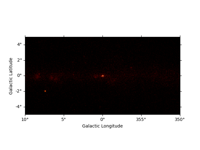
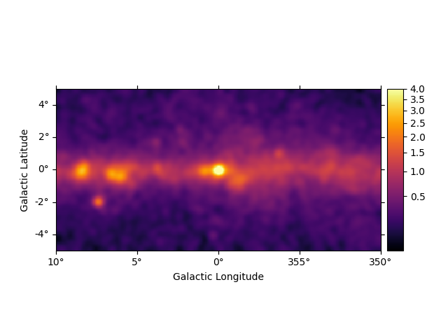
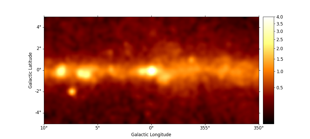
We can easily improve the plot by calling smooth() first and providing additional arguments to plot(). Most of them are passed further to plt.imshow():

smoothed = m_3fhl_gc.smooth(width=0.2 * u.deg, kernel="gauss")
smoothed.plot(stretch="sqrt", add_cbar=True, vmax=4, cmap="inferno")
plt.show()

We can use the plt.rc_context() context manager to further tweak the plot by adapting the figure and font size:

rc_params = {"figure.figsize": (12, 5.4), "font.size": 12}
with plt.rc_context(rc=rc_params):
    smoothed = m_3fhl_gc.smooth(width=0.2 * u.deg, kernel="gauss")
    smoothed.plot(stretch="sqrt", add_cbar=True, vmax=4)
plt.show()

Cube plotting

For maps with non-spatial dimensions the Map object features an interactive plotting method, that works in jupyter notebooks only (Note: it requires the package ipywidgets to be installed). We first read a small example cutout from the Fermi Galactic diffuse model and display the data cube by calling plot_interactive():

rc_params = {
    "figure.figsize": (12, 5.4),
    "font.size": 12,
    "axes.formatter.limits": (2, -2),
}
m_iem_gc.plot_interactive(add_cbar=True, stretch="sqrt", rc_params=rc_params)
plt.show()

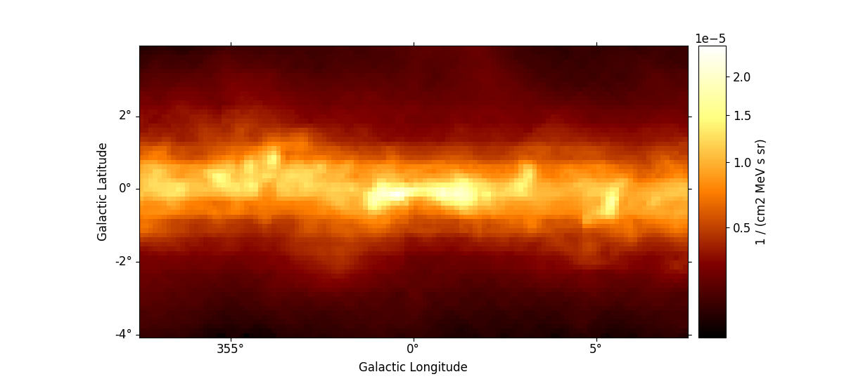
interactive(children=(SelectionSlider(continuous_update=False, description='Select energy_true:', layout=Layout(width='50%'), options=('58.5 MeV', '80.0 MeV', '109 MeV', '150 MeV', '205 MeV', '280 MeV', '383 MeV', '523 MeV', '716 MeV', '979 MeV', '1.34 GeV', '1.83 GeV', '2.50 GeV', '3.42 GeV', '4.68 GeV', '6.41 GeV', '8.76 GeV', '12.0 GeV', '16.4 GeV', '22.4 GeV', '30.6 GeV', '41.9 GeV', '57.3 GeV', '78.4 GeV', '107 GeV', '147 GeV', '201 GeV', '274 GeV', '375 GeV', '513 GeV'), style=SliderStyle(description_width='initial'), value='58.5 MeV'), RadioButtons(description='Select stretch:', index=1, options=('linear', 'sqrt', 'log'), style=DescriptionStyle(description_width='initial'), value='sqrt'), Output()), _dom_classes=('widget-interact',))

Now you can use the interactive slider to select an energy range and the corresponding image is displayed on the screen. You can also use the radio buttons to select your preferred image stretching. We have passed additional keywords using the rc_params argument to improve the figure and font size. Those keywords are directly passed to the plt.rc_context() context manager.

Additionally all the slices of a 3D Map can be displayed using the plot_grid() method. By default the colorbars bounds of the subplots are not the same, we can make them consistent using the vmin and vmax options:

counts_3d.plot_grid(ncols=4, figsize=(16, 12), vmin=0, vmax=100, stretch="log")
plt.show()