Note
Go to the end to download the full example code. or to run this example in your browser via Binder
Fitting#
Learn how the model, dataset and fit Gammapy classes work together in a detailed modeling and fitting use-case.
Note#
This tutorial describes the fitting steps using a maximum likelihood (Frequentist approach).
Alternatively, we could have a Bayesian approach by assigning a prior probability distribution over the parameters and compute the posterior distribution to fit the parameters. This is described in the Priors tutorial.
One can also perform a Bayesian analysis using a nested sampling technique. This is described in the Bayesian analysis with nested sampling tutorial.
Prerequisites#
Knowledge of spectral analysis to produce 1D On-Off datasets, see the Spectral analysis tutorial.
Reading of pre-computed datasets see e.g. Multi instrument joint 3D and 1D analysis tutorial.
General knowledge on statistics and optimization methods
Proposed approach#
This is a hands-on tutorial to modeling, showing how to do
perform a Fit in gammapy. The emphasis here is on interfacing the
Fit class and inspecting the errors. To see an analysis example of
how datasets and models interact, see the Modelling tutorial.
As an example, in this notebook, we are going to work with H.E.S.S. data of the Crab Nebula and show in
particular how to :
perform a spectral analysis
use different fitting backends
access covariance matrix information and parameter errors
compute likelihood profile - compute confidence contours
See also: Models and Modeling and Fitting (DL4 to DL5).
The setup#
from itertools import combinations
import numpy as np
from astropy import units as u
import matplotlib.pyplot as plt
from IPython.display import display
from gammapy.datasets import Datasets, SpectrumDatasetOnOff
from gammapy.modeling import Fit
from gammapy.modeling.models import LogParabolaSpectralModel, SkyModel
Check setup#
from gammapy.utils.check import check_tutorials_setup
from gammapy.visualization.utils import plot_contour_line

check_tutorials_setup()
System:

        python_executable      : /home/runner/work/gammapy-docs/gammapy-docs/gammapy/.tox/build_docs/bin/python
        python_version         : 3.9.22
        machine                : x86_64
        system                 : Linux


Gammapy package:

        version                : 2.0.dev1166+g47b6a2f52
        path                   : /home/runner/work/gammapy-docs/gammapy-docs/gammapy/.tox/build_docs/lib/python3.9/site-packages/gammapy


Other packages:

        numpy                  : 1.26.4
        scipy                  : 1.13.1
        astropy                : 6.0.1
        regions                : 0.8
        click                  : 8.1.8
        yaml                   : 6.0.2
        IPython                : 8.18.1
        jupyterlab             : not installed
        matplotlib             : 3.9.4
        pandas                 : not installed
        healpy                 : 1.17.3
        iminuit                : 2.31.1
        sherpa                 : 4.16.1
        naima                  : 0.10.0
        emcee                  : 3.1.6
        corner                 : 2.2.3
        ray                    : 2.46.0


Gammapy environment variables:

        GAMMAPY_DATA           : /home/runner/work/gammapy-docs/gammapy-docs/gammapy-datasets/dev
Model and dataset#
First we define the source model, here we need only a spectral model for which we choose a log-parabola
crab_spectrum = LogParabolaSpectralModel(
    amplitude=1e-11 / u.cm**2 / u.s / u.TeV,
    reference=1 * u.TeV,
    alpha=2.3,
    beta=0.2,
)

crab_spectrum.alpha.max = 3
crab_spectrum.alpha.min = 1
crab_model = SkyModel(spectral_model=crab_spectrum, name="crab")
The data and background are read from pre-computed ON/OFF datasets of H.E.S.S. observations, for simplicity we stack them together. Then we set the model and fit range to the resulting dataset.
datasets = []
for obs_id in [23523, 23526]:
    dataset = SpectrumDatasetOnOff.read(
        f"$GAMMAPY_DATA/joint-crab/spectra/hess/pha_obs{obs_id}.fits"
    )
    datasets.append(dataset)

dataset_hess = Datasets(datasets).stack_reduce(name="HESS")
datasets = Datasets(datasets=[dataset_hess])

# Set model and fit range
dataset_hess.models = crab_model
e_min = 0.66 * u.TeV
e_max = 30 * u.TeV
dataset_hess.mask_fit = dataset_hess.counts.geom.energy_mask(e_min, e_max)
Fitting options#
First let’s create a Fit instance:
scipy_opts = {
    "method": "L-BFGS-B",
    "options": {"ftol": 1e-4, "gtol": 1e-05},
    "backend": "scipy",
}
fit_scipy = Fit(store_trace=True, optimize_opts=scipy_opts)
By default the fit is performed using MINUIT, you can select alternative
optimizers and set their option using the optimize_opts argument of
the Fit.run() method. In addition we have specified to store the
trace of parameter values of the fit.
Note that, for now, covariance matrix and errors are computed only for the fitting with MINUIT. However, depending on the problem other optimizers can better perform, so sometimes it can be useful to run a pre-fit with alternative optimization methods.
sherpa_opts = {"method": "simplex", "ftol": 1e-3, "maxfev": int(1e4)}
fit_sherpa = Fit(store_trace=True, backend="sherpa", optimize_opts=sherpa_opts)
results_simplex = fit_sherpa.run(datasets)
For the “minuit” backend see https://iminuit.readthedocs.io/en/latest/reference.html for a detailed description of the available options. If there is an entry ‘migrad_opts’, those options will be passed to iminuit.Minuit.migrad. Additionally you can set the fit tolerance using the tol option. The minimization will stop when the estimated distance to the minimum is less than 0.001*tol (by default tol=0.1). The strategy option change the speed and accuracy of the optimizer: 0 fast, 1 default, 2 slow but accurate. If you want more reliable error estimates, you should run the final fit with strategy 2.
fit = Fit(store_trace=True)
minuit_opts = {"tol": 0.001, "strategy": 1}
fit.backend = "minuit"
fit.optimize_opts = minuit_opts
result_minuit = fit.run(datasets)
Fit quality assessment#
There are various ways to check the convergence and quality of a fit. Among them:
Refer to the automatically-generated results dictionary:
print(result_scipy)
OptimizeResult

        backend    : scipy
        method     : L-BFGS-B
        success    : True
        message    : CONVERGENCE: REL_REDUCTION_OF_F_<=_FACTR*EPSMCH
        nfev       : 60
        total stat : 30.35

CovarianceResult

        backend    : minuit
        method     : hesse
        success    : True
        message    : Hesse terminated successfully.
print(results_simplex)
OptimizeResult

        backend    : sherpa
        method     : simplex
        success    : True
        message    : Optimization terminated successfully
        nfev       : 135
        total stat : 30.35
print(result_minuit)
OptimizeResult

        backend    : minuit
        method     : migrad
        success    : True
        message    : Optimization terminated successfully.
        nfev       : 37
        total stat : 30.35

CovarianceResult

        backend    : minuit
        method     : hesse
        success    : True
        message    : Hesse terminated successfully.
If the fit is performed with minuit you can print detailed information to check the convergence
print(result_minuit.minuit)
┌─────────────────────────────────────────────────────────────────────────┐
│                                Migrad                                   │
├──────────────────────────────────┬──────────────────────────────────────┤
│ FCN = 30.35                      │              Nfcn = 37               │
│ EDM = 3.42e-08 (Goal: 2e-06)     │            time = 0.2 sec            │
├──────────────────────────────────┼──────────────────────────────────────┤
│          Valid Minimum           │   Below EDM threshold (goal x 10)    │
├──────────────────────────────────┼──────────────────────────────────────┤
│      No parameters at limit      │           Below call limit           │
├──────────────────────────────────┼──────────────────────────────────────┤
│             Hesse ok             │         Covariance accurate          │
└──────────────────────────────────┴──────────────────────────────────────┘
┌───┬───────────────────┬───────────┬───────────┬────────────┬────────────┬─────────┬─────────┬───────┐
│   │ Name              │   Value   │ Hesse Err │ Minos Err- │ Minos Err+ │ Limit-  │ Limit+  │ Fixed │
├───┼───────────────────┼───────────┼───────────┼────────────┼────────────┼─────────┼─────────┼───────┤
│ 0 │ par_000_amplitude │    3.8    │    0.4    │            │            │         │         │       │
│ 1 │ par_001_alpha     │   2.20    │   0.26    │            │            │    1    │    3    │       │
│ 2 │ par_002_beta      │    2.3    │    1.4    │            │            │         │         │       │
└───┴───────────────────┴───────────┴───────────┴────────────┴────────────┴─────────┴─────────┴───────┘
┌───────────────────┬───────────────────────────────────────────────────────┐
│                   │ par_000_amplitude     par_001_alpha      par_002_beta │
├───────────────────┼───────────────────────────────────────────────────────┤
│ par_000_amplitude │             0.126              0.05             -0.12 │
│     par_001_alpha │              0.05            0.0689             -0.33 │
│      par_002_beta │             -0.12             -0.33              1.95 │
└───────────────────┴───────────────────────────────────────────────────────┘
Check the trace of the fit e.g. in case the fit did not converge properly
display(result_minuit.trace)
    total_stat     crab.spectral.amplitude ...  crab.spectral.beta
------------------ ----------------------- ... -------------------
30.349530550364513  3.8122425528751894e-11 ...  0.2264827221149211
30.349724385715966   3.815791997446166e-11 ...  0.2264827221149211
30.349711555166778   3.808693108304212e-11 ...  0.2264827221149211
30.349539326364486   3.812951376050203e-11 ...  0.2264827221149211
30.349536722980144   3.811533729700176e-11 ...  0.2264827221149211
 30.35050396342807  3.8122425528751894e-11 ...  0.2264827221149211
 30.35053891085894  3.8122425528751894e-11 ...  0.2264827221149211
30.349538946234787  3.8122425528751894e-11 ...  0.2264827221149211
30.349541972204694  3.8122425528751894e-11 ...  0.2264827221149211
30.350292033852874  3.8122425528751894e-11 ... 0.22788666362099286
               ...                     ... ...                 ...
30.349537804335895    3.81221696315049e-11 ... 0.22662623775461227
 30.34953807800248    3.81221696315049e-11 ... 0.22635141851205703
30.349530774637106  3.8123587278110435e-11 ... 0.22648882813333465
 30.34953075814257  3.8120751984899354e-11 ... 0.22648882813333465
30.349530807499818    3.81221696315049e-11 ... 0.22648882813333465
30.349530725238324    3.81221696315049e-11 ... 0.22648882813333465
30.349530739434762    3.81221696315049e-11 ... 0.22651631005759018
30.349530793294022    3.81221696315049e-11 ... 0.22646134620907912
30.349535814771492    3.81292578645326e-11 ... 0.22648882813333465
 30.34953715852974    3.81292578645326e-11 ... 0.22662623775461227
30.349559366767238    3.81221696315049e-11 ... 0.22662623775461227
Length = 37 rows
The fitted models are copied on the FitResult object.
They can be inspected to check that the fitted values and errors
for all parameters are reasonable, and no fitted parameter value is “too close”
- or even outside - its allowed min-max range
display(result_minuit.models.to_parameters_table())
model type    name     value         unit      ...    max    frozen link prior
----- ---- --------- ---------- -------------- ... --------- ------ ---- -----
 crab      amplitude 3.8122e-11 TeV-1 s-1 cm-2 ...       nan  False
 crab      reference 1.0000e+00            TeV ...       nan   True
 crab          alpha 2.1958e+00                ... 3.000e+00  False
 crab           beta 2.2649e-01                ...       nan  False
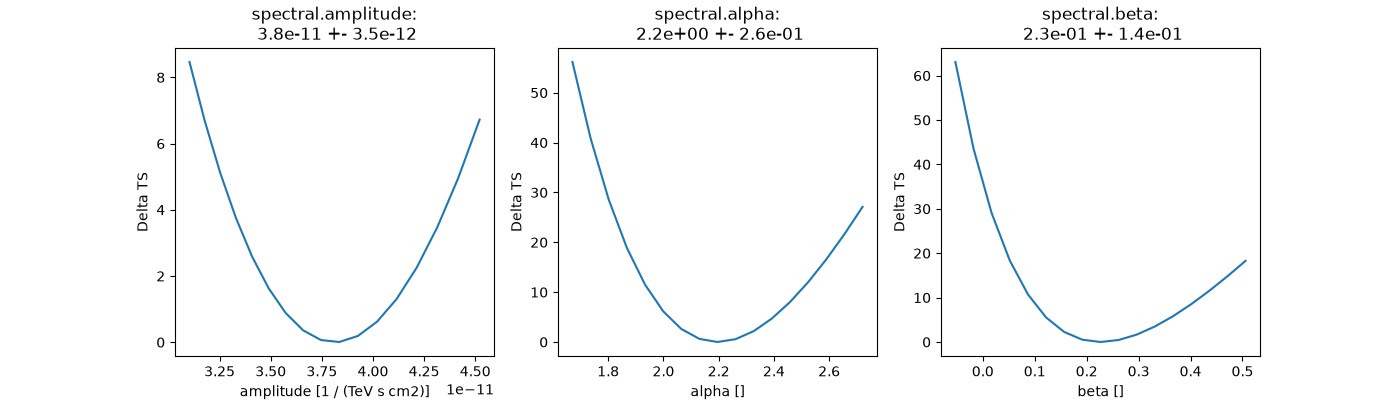
Plot fit statistic profiles for all fitted parameters, using
stat_profile. For a good fit and error
estimate each profile should be parabolic. The specification for each
fit statistic profile can be changed on the
Parameter object, which has scan_min,
scan_max, scan_n_values and scan_n_sigma attributes.
total_stat = result_minuit.total_stat

fig, axes = plt.subplots(nrows=1, ncols=3, figsize=(14, 4))

for ax, par in zip(axes, crab_model.parameters.free_parameters):
    par.scan_n_values = 17
    idx = crab_model.parameters.index(par)
    name = crab_model.parameters_unique_names[idx]
    profile = fit.stat_profile(datasets=datasets, parameter=par)
    ax.plot(
        profile[f"{crab_model.name}.{name}_scan"], profile["stat_scan"] - total_stat
    )
    ax.set_xlabel(f"{par.name} [{par.unit}]")
    ax.set_ylabel("Delta TS")
    ax.set_title(f"{name}:\n {par.value:.1e} +- {par.error:.1e}")
plt.show()
Inspect model residuals. Those can always be accessed using
residuals(). For more details, we refer here to the dedicated
3D detailed analysis (for MapDataset fitting) and
Spectral analysis (for SpectrumDataset fitting).
Covariance and parameters errors#
After the fit the covariance matrix is attached to the models copy
stored on the FitResult object.
You can access it directly with:
[[ 1.25743552e-23  0.00000000e+00  4.54676809e-13 -1.17016467e-13]
 [ 0.00000000e+00  0.00000000e+00  0.00000000e+00  0.00000000e+00]
 [ 4.54676809e-13  0.00000000e+00  6.89492101e-02 -3.31139055e-02]
 [-1.17016467e-13  0.00000000e+00 -3.31139055e-02  1.95024536e-02]]
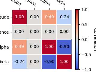
And you can plot the total parameter correlation as well:
result_minuit.models.covariance.plot_correlation(figsize=(7, 5))
plt.show()
The covariance information is also propagated to the individual models
Therefore, one can also get the error on a specific parameter by directly
accessing the error attribute:
0.26258181596485647
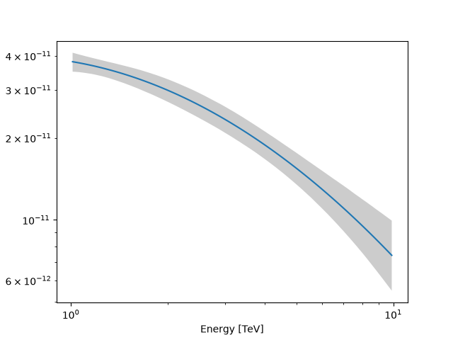
As an example, this step is needed to produce a butterfly plot showing the envelope of the model taking into account parameter uncertainties.
energy_bounds = [1, 10] * u.TeV
crab_spectrum.plot(energy_bounds=energy_bounds, energy_power=2)
ax = crab_spectrum.plot_error(energy_bounds=energy_bounds, energy_power=2)
plt.show()
Confidence contours#
In most studies, one wishes to estimate parameters distribution using observed sample data. A 1-dimensional confidence interval gives an estimated range of values which is likely to include an unknown parameter. A confidence contour is a 2-dimensional generalization of a confidence interval, often represented as an ellipsoid around the best-fit value.
Gammapy offers two ways of computing confidence contours, in the
dedicated methods stat_contour and stat_profile. In
the following sections we will describe them.
An important point to keep in mind is: what does a
Computing contours using stat_contour#
After the fit, MINUIT offers the possibility to compute the confidence
contours. gammapy provides an interface to this functionality through
the Fit object using the stat_contour method. Here we defined a
function to automate the contour production for the different
parameter and confidence levels (expressed in terms of sigma):
def make_contours(fit, datasets, model, params, npoints, sigmas):
    cts_sigma = []
    for sigma in sigmas:
        contours = dict()
        for par_1, par_2 in combinations(params, r=2):
            idx1, idx2 = model.parameters.index(par_1), model.parameters.index(par_2)
            name1 = model.parameters_unique_names[idx1]
            name2 = model.parameters_unique_names[idx2]
            contour = fit.stat_contour(
                datasets=datasets,
                x=model.parameters[par_1],
                y=model.parameters[par_2],
                numpoints=npoints,
                sigma=sigma,
            )
            contours[f"contour_{par_1}_{par_2}"] = {
                par_1: contour[f"{model.name}.{name1}"].tolist(),
                par_2: contour[f"{model.name}.{name2}"].tolist(),
            }
        cts_sigma.append(contours)
    return cts_sigma
Now we can compute few contours.
Define the combinations of parameters to plot
param_pairs = list(combinations(params, r=2))
Labels for plotting
labels = {
    "amplitude": r"$\phi_0 \,/\,({\rm TeV}^{-1} \, {\rm cm}^{-2} {\rm s}^{-1})$",
    "alpha": r"$\alpha$",
    "beta": r"$\beta$",
}
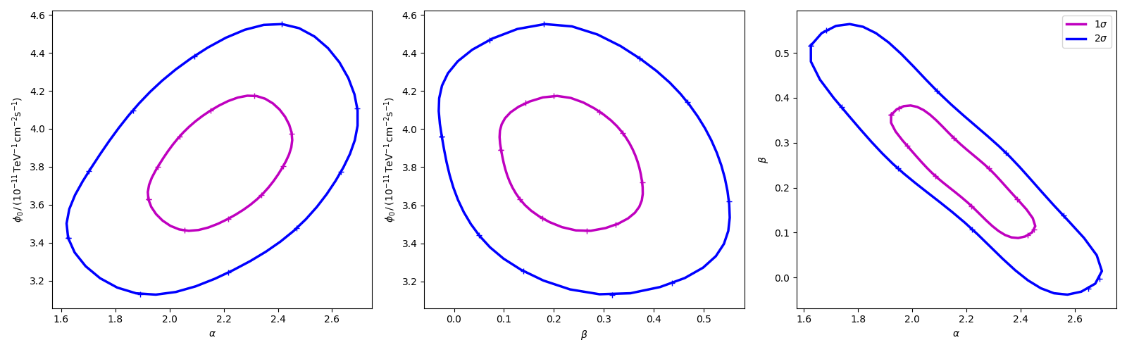
Produce the confidence contours figures.
fig, axes = plt.subplots(1, 3, figsize=(10, 3))
colors = ["m", "b", "c"]

for (par_1, par_2), ax in zip(param_pairs, axes):
    for ks, sigma in enumerate(sigmas):
        contour = cts_sigma[ks][f"contour_{par_1}_{par_2}"]
        plot_contour_line(
            ax,
            contour[par_1],
            contour[par_2],
            lw=2.5,
            color=colors[ks],
            label=f"{sigmas[ks]}" + r"$\sigma$",
        )
    ax.set_xlabel(labels[par_1])
    ax.set_ylabel(labels[par_2])
plt.legend()
plt.tight_layout()
Computing contours using stat_surface#
This alternative method for the computation of confidence contours,
although more time consuming than stat_contour(), is expected
to be more stable. It consists of a generalization of
stat_profile() to a 2-dimensional parameter space. The algorithm
is very simple: - First, passing two arrays of parameters values, a
2-dimensional discrete parameter space is defined; - For each node of
the parameter space, the two parameters of interest are frozen. This
way, a likelihood value (
Let’s see it step by step.
First of all, we can notice that this method is “backend-agnostic”, meaning that it can be run with MINUIT, sherpa or scipy as fitting tools. Here we will stick with MINUIT, which is the default choice:
As an example, we can compute the confidence contour for the alpha
and beta parameters of the dataset_hess. Here we define the
parameter space:
result = result_minuit
par_alpha = crab_model.parameters["alpha"]
par_beta = crab_model.parameters["beta"]

par_alpha.scan_values = np.linspace(1.55, 2.7, 20)
par_beta.scan_values = np.linspace(-0.05, 0.55, 20)
Then we run the algorithm, by choosing reoptimize=False for the sake
of time saving. In real life applications, we strongly recommend to use
reoptimize=True, so that all free nuisance parameters will be fit at
each grid node. This is the correct way, statistically speaking, of
computing confidence contours, but is expected to be time consuming.
fit = Fit(backend="minuit", optimize_opts={"print_level": 0})
stat_surface = fit.stat_surface(
    datasets=datasets,
    x=par_alpha,
    y=par_beta,
    reoptimize=False,
)
In order to easily inspect the results, we can convert the
# Compute TS
TS = stat_surface["stat_scan"] - result.total_stat

# Compute the corresponding statistical significance surface
stat_surface = np.sqrt(TS.T)
Notice that, as explained before,
# Compute the corresponding statistical significance surface
# p_value = 1 - st.chi2(df=1).cdf(TS)
# gaussian_sigmas = st.norm.isf(p_value / 2).T
Finally, we can plot the surface values together with contours:
fig, ax = plt.subplots(figsize=(8, 6))
x_values = par_alpha.scan_values
y_values = par_beta.scan_values

# plot surface
im = ax.pcolormesh(x_values, y_values, stat_surface, shading="auto")
fig.colorbar(im, label="sqrt(TS)")
ax.set_xlabel(f"{par_alpha.name}")
ax.set_ylabel(f"{par_beta.name}")

# We choose to plot 1 and 2 sigma confidence contours
levels = [1, 2]
contours = ax.contour(x_values, y_values, stat_surface, levels=levels, colors="white")
ax.clabel(contours, fmt="%.0f $\\sigma$", inline=3, fontsize=15)

plt.show()
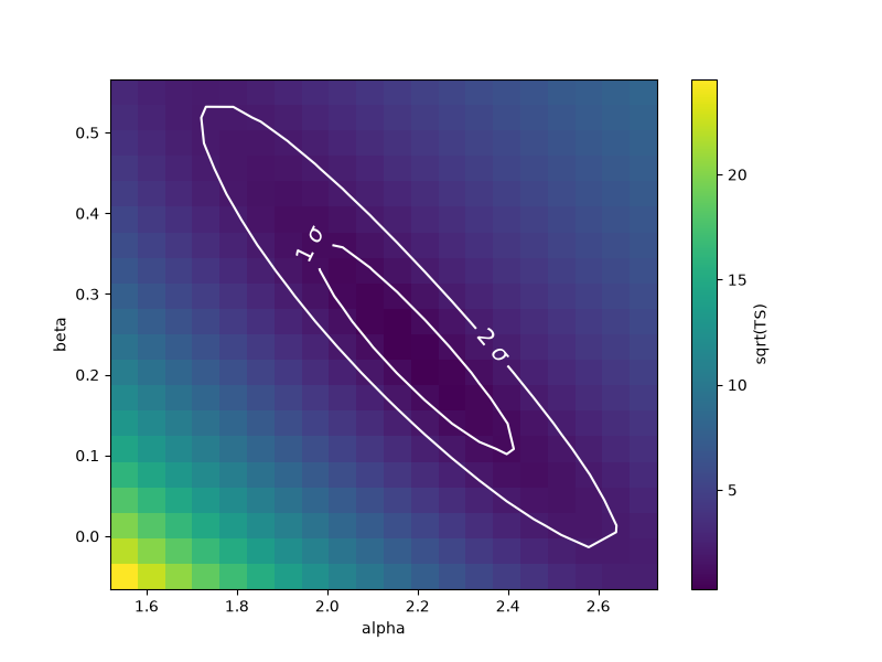
Note that, if computed with reoptimize=True, this plot would be
completely consistent with the third panel of the plot produced with
stat_contour (try!).
Finally, it is always remember that confidence contours are approximations. In particular, when the parameter range boundaries are close to the contours lines, it is expected that the statistical meaning of the contours is not well defined. That’s why we advise to always choose a parameter space that contains the contours you’re interested in.
Total running time of the script: (0 minutes 27.126 seconds)