Mask maps

Create and apply masks maps.

Prerequisites

• Understanding of basic analyses in 1D or 3D.

• Usage of regions and catalogs, see the catalog notebook.

Context

There are two main categories of masks in Gammapy for different use cases. - Fitting often requires to ignore some parts of a reduced dataset, e.g. to restrict the fit to a specific energy range or to ignore parts of the region of interest that the user does not want to model, or both. Gammapy’s Datasets therefore contain a mask_fit sharing the same geometry as the data (i.e. counts). - During data reduction, some background makers will normalize the background model template on the data themselves. To limit contamination by real photons, one has to exclude parts of the field-of-view where signal is expected to be large. To do so, one needs to provide an exclusion mask. The latter can be provided in a different geometry as it will be reprojected by the Makers.

We explain in more details these two types of masks below:

Masks for fitting

The region of interest used for the fit can defined through the dataset mask_fit attribute. The mask_fit is a map containing boolean values where pixels used in the fit are stored as True.

A spectral fit (1D or 3D) can be restricted to a specific energy range where e.g. the background is well estimated or where the number of counts is large enough. Similarly, 2D and 3D analyses usually require to work with a wider map than the region of interest so sources laying outside but reconstructed inside because of the PSF are correctly taken into account. Then the mask_fit have to include a margin that take into account the PSF width. We will show an example in the boundary mask sub-section.

The mask_fit also can be used to exclude sources or complex regions for which we don’t have good enough models. In that case the masking is an extra security, it is preferable to include the available models even if the sources are masked and frozen.

Note that a dataset contains also a mask_safe attribute that is created and filled during data reduction. It is not to be modified directly by users. The mask_safe is defined only from the options passed to the SafeMaskMaker.

Exclusion masks

Background templates stored in the DL3 IRF are often not reliable enough to be used without some corrections. A set of common techniques to perform background or normalisation from the data is implemented in gammapy: reflected regions for 1D spectrum analysis, field-of-view (FoV) background or ring background for 2D and 3D analyses.

To avoid contamination of the background estimate from gamma-ray bright regions these methods require to exclude those regions from the data used for the estimation. To do so, we use exclusion masks. They are maps containing boolean values where excluded pixels are stored as False.

Proposed approach

Even if the use cases for exclusion masks and fit masks are different, the way to create these masks is exactly the same, so in the following we show how to work with masks in general:

• Creating masks from scratch

• Combining multiple masks

• Extending and reducing an existing mask

• Reading and writing masks

Setup

import numpy as np
import astropy.units as u
from astropy.coordinates import Angle, SkyCoord
from regions import CircleSkyRegion, Regions

# %matplotlib inline
import matplotlib.pyplot as plt
from gammapy.catalog import CATALOG_REGISTRY
from gammapy.datasets import Datasets
from gammapy.estimators import ExcessMapEstimator
from gammapy.maps import Map, WcsGeom

Check setup

from gammapy.utils.check import check_tutorials_setup

check_tutorials_setup()

System:

        python_executable      : /home/runner/work/gammapy-docs/gammapy-docs/gammapy/.tox/build_docs/bin/python
        python_version         : 3.9.20
        machine                : x86_64
        system                 : Linux


Gammapy package:

        version                : 2.0.dev155+g9309a089d
        path                   : /home/runner/work/gammapy-docs/gammapy-docs/gammapy/.tox/build_docs/lib/python3.9/site-packages/gammapy


Other packages:

        numpy                  : 1.26.4
        scipy                  : 1.13.1
        astropy                : 5.2.2
        regions                : 0.8
        click                  : 8.1.7
        yaml                   : 6.0.2
        IPython                : 8.18.1
        jupyterlab             : not installed
        matplotlib             : 3.9.4
        pandas                 : not installed
        healpy                 : 1.17.3
        iminuit                : 2.30.1
        sherpa                 : 4.16.1
        naima                  : 0.10.0
        emcee                  : 3.1.6
        corner                 : 2.2.3
        ray                    : 2.40.0


Gammapy environment variables:

        GAMMAPY_DATA           : /home/runner/work/gammapy-docs/gammapy-docs/gammapy-datasets/dev

Creating a mask for fitting

One can build a mask_fit to restrict the energy range of pixels used to fit a Dataset. The mask being a Map it needs to use the same geometry (i.e. a Geom object) as the Dataset it will be applied to.

We show here how to proceed on a MapDataset taken from Fermi data used in the 3FHL catalog. The dataset is already in the form of a Datasets object. We read it from disk.

filename = "$GAMMAPY_DATA/fermi-3fhl-crab/Fermi-LAT-3FHL_datasets.yaml"
datasets = Datasets.read(filename=filename)
dataset = datasets["Fermi-LAT"]

We can check the default energy range of the dataset. In the absence of a mask_fit it is equal to the safe energy range.

print(f"Fit range : {dataset.energy_range_total}")

Fit range : (<Quantity 0.01 TeV>, <Quantity 2. TeV>)

Create a mask in energy

We show first how to use a simple helper function energy_range().

We obtain the Geom that is stored on the counts map inside the Dataset and we can directly create the Map.

mask_energy = dataset.counts.geom.energy_mask(10 * u.GeV, 700 * u.GeV)

We can now set the dataset mask_fit attribute.

And we check that the total fit range has changed accordingly. The bin edges closest to requested range provide the actual fit range.

dataset.mask_fit = mask_energy
print(f"Fit range : {dataset.energy_range_total}")

Fit range : (<Quantity 0.028854 TeV>, <Quantity 0.69314486 TeV>)

Mask some sky regions

One might also exclude some specific part of the sky for the fit. For instance, if one wants not to model a specific source in the region of interest, or if one want to reduce the region of interest in the dataset Geom.

In the following we restrict the fit region to a square around the Crab nebula. Note: the dataset geometry is aligned on the galactic frame, we use the same frame to define the box to ensure a correct alignment. We can now create the map. We use the WcsGeom.region_mask method putting all pixels outside the regions to False (because we only want to consider pixels inside the region. For convenience, we can directly pass a ds9 region string to the method:

regions = "galactic;box(184.55, -5.78, 3.0, 3.0)"
mask_map = dataset.counts.geom.region_mask(regions)

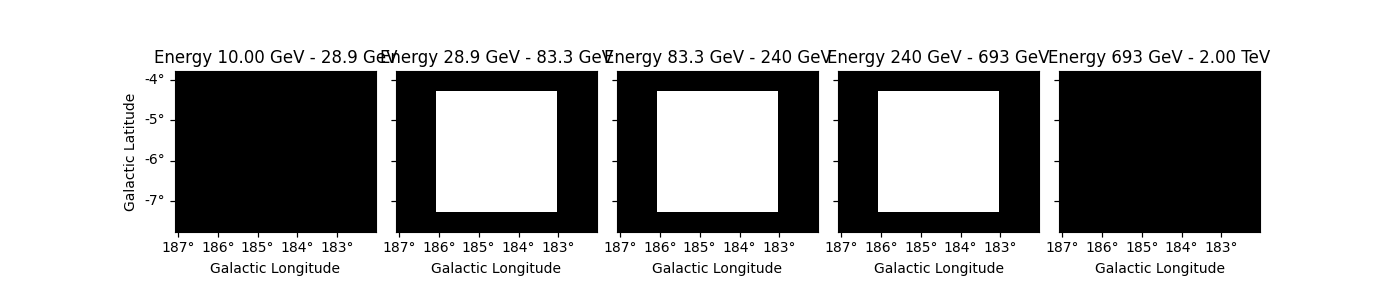
We can now combine this mask with the energy mask using the logical and operator

dataset.mask_fit &= mask_map

Let’s check the result and plot the full mask.

dataset.mask_fit.plot_grid(ncols=5, vmin=0, vmax=1, figsize=(14, 3))
plt.show()

Creating a mask manually

If you are more familiar with the Geom and Map API, you can also create the mask manually from the coordinates of all pixels in the geometry. Here we simply show how to obtain the same behaviour as the energy_mask helper method.

In practice, this allows to create complex energy dependent masks.

coords = dataset.counts.geom.get_coord()
mask_data = (coords["energy"] >= 10 * u.GeV) & (coords["energy"] < 700 * u.GeV)
mask_energy = Map.from_geom(dataset.counts.geom, data=mask_data)

Creating an exclusion mask

Exclusion masks are typically used for background estimation to mask out regions where gamma-ray signal is expected. An exclusion mask is usually a simple 2D boolean Map where excluded positions are stored as False. Their actual geometries are independent of the target datasets that a user might want to build. The first thing to do is to build the geometry.

Define the geometry

Masks are stored in Map objects. We must first define its geometry and then we can determine which pixels to exclude. Here we consider a region at the Galactic anti-centre around the crab nebula.

position = SkyCoord(83.633083, 22.0145, unit="deg", frame="icrs")
geom = WcsGeom.create(skydir=position, width="5 deg", binsz=0.02, frame="galactic")

Create the mask from a list of regions

One can build an exclusion mask from regions. We show here how to proceed.

We can rely on known sources positions and properties to build a list of regions (here SkyRegions) enclosing most of the signal that our detector would see from these objects.

A useful function to create region objects is parse. It can take strings defining regions e.g. following the “ds9” format and convert them to regions.

Here we use a region enclosing the Crab nebula with 0.3 degrees. The actual region size should depend on the expected PSF of the data used. We also add another region with a different shape as en example.

regions_ds9 = "galactic;box(185,-4,1.0,0.5, 45);icrs;circle(83.633083, 22.0145, 0.3)"
regions = Regions.parse(regions_ds9, format="ds9")
print(regions)

[<RectangleSkyRegion(center=<SkyCoord (Galactic): (l, b) in deg
    (185., -4.)>, width=1.0 deg, height=0.5 deg, angle=45.0 deg)>, <CircleSkyRegion(center=<SkyCoord (ICRS): (ra, dec) in deg
    (83.633083, 22.0145)>, radius=0.3 deg)>]

Equivalently the regions can be read from a ds9 file, this time using Regions.read.

# regions = Regions.read('ds9.reg', format="ds9")

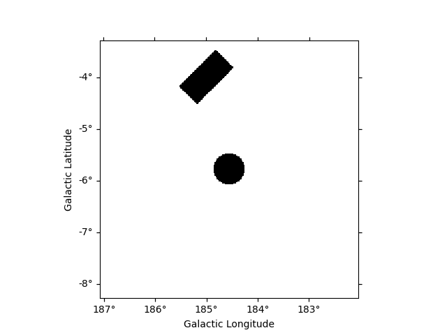
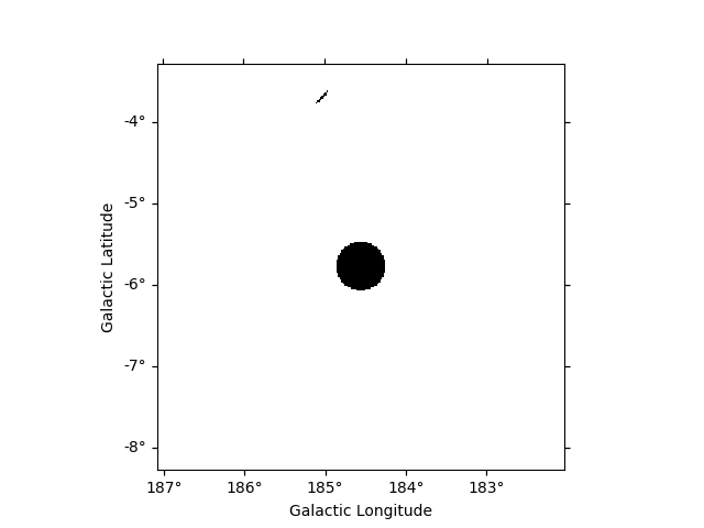
Create the mask map

We can now create the map. We use the WcsGeom.region_mask method putting all pixels inside the regions to False.

# to define the exclusion mask we take the inverse
mask_map = ~geom.region_mask(regions)
mask_map.plot()
plt.show()

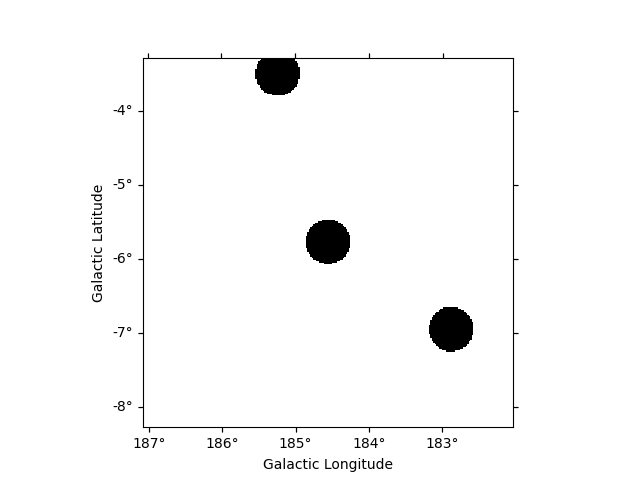
Create the mask from a catalog of sources

We can also build our list of regions from a list of catalog sources. Here we use the Fermi 4FGL catalog which we read using SourceCatalog.

fgl = CATALOG_REGISTRY.get_cls("4fgl")()

We now select sources that are contained in the region we are interested in.

inside_geom = geom.contains(fgl.positions)
positions = fgl.positions[inside_geom]

We now create the list of regions using our 0.3 degree radius a priori value. If the sources were extended, one would have to adapt the sizes to account for the larger size.

exclusion_radius = Angle("0.3 deg")
regions = [CircleSkyRegion(position, exclusion_radius) for position in positions]

Now we can build the mask map the same way as above.

mask_map_catalog = ~geom.region_mask(regions)
mask_map_catalog.plot()
plt.show()

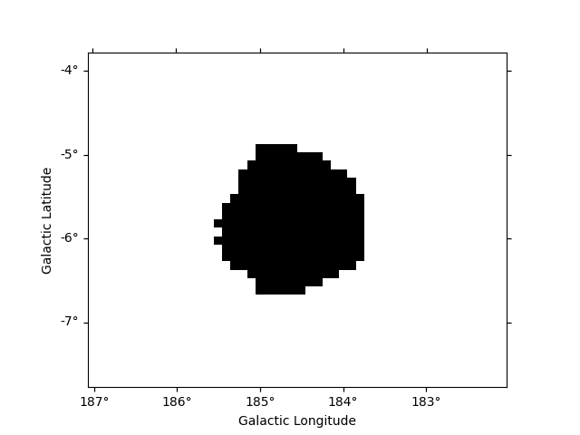
Create the mask from statistically significant pixels in a dataset

Here we want to determine an exclusion from the data directly. We will estimate the significance of the data using the ExcessMapEstimator, and exclude all pixels above a given threshold.

Here we use the MapDataset taken from the Fermi data used above.

We apply a significance estimation. We integrate the counts using a correlation radius of 0.4 degree and apply regular significance estimate.

estimator = ExcessMapEstimator("0.4 deg", selection_optional=[])
result = estimator.run(dataset)

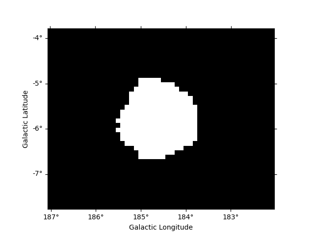
Finally, we create the mask map by applying a threshold of 5 sigma to remove pixels.

significance_mask = result["sqrt_ts"] < 5.0

Because the ExcessMapEstimator returns NaN for masked pixels, we need to put the NaN values to True to avoid incorrectly excluding them.

invalid_pixels = np.isnan(result["sqrt_ts"].data)
significance_mask.data[invalid_pixels] = True
significance_mask.plot()
plt.show()

This method frequently yields isolated pixels or weakly significant features if one places the threshold too low.

To overcome this issue, one can use apply_hysteresis_threshold . This filter allows to define two thresholds and mask only the pixels between the low and high thresholds if they are not continuously connected to a pixel above the high threshold. This allows to better preserve the structure of the excesses.

Note that scikit-image is not a required dependency of gammapy, you might need to install it.

Masks operations

If two masks share the same geometry it is easy to combine them with Map arithmetic.

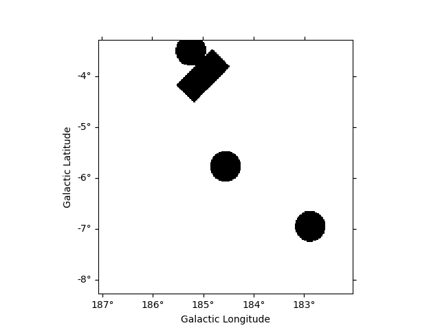
OR condition is represented by | operator :

mask = mask_map | mask_map_catalog
mask.plot()
plt.show()

AND condition is represented by & or * operators :

mask_map &= mask_map_catalog
mask_map.plot()
plt.show()

The NOT operator is represented by the ~ symbol:

significance_mask_inv = ~significance_mask
significance_mask_inv.plot()
plt.show()

Mask modifications

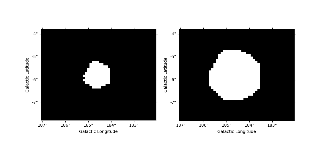
Mask dilation and erosion

One can reduce or extend a mask using binary_erode and binary_dilate methods, respectively.

fig, (ax1, ax2) = plt.subplots(
    figsize=(11, 5), ncols=2, subplot_kw={"projection": significance_mask_inv.geom.wcs}
)

mask = significance_mask_inv.binary_erode(width=0.2 * u.deg, kernel="disk")
mask.plot(ax=ax1)

mask = significance_mask_inv.binary_dilate(width=0.2 * u.deg)
mask.plot(ax=ax2)
plt.show()

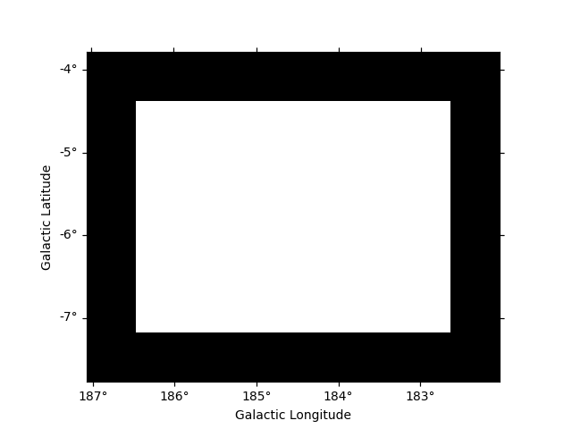
Boundary mask

In the following example we use the Fermi dataset previously loaded and add its mask_fit taking into account a margin based on the psf width. The margin width is determined using the containment_radius method of the psf object and the mask is created using the boundary_mask method available on the geometry object.

# get PSF 95% containment radius
energy_true = dataset.exposure.geom.axes[0].center
psf_r95 = dataset.psf.containment_radius(fraction=0.95, energy_true=energy_true)
plt.show()

# create mask_fit with margin based on PSF
mask_fit = dataset.counts.geom.boundary_mask(psf_r95.max())
dataset.mask_fit = mask_fit
dataset.mask_fit.sum_over_axes().plot()
plt.show()

Reading and writing masks

gammapy.maps can directly read/write maps with boolean content as follows:

# To save masks to disk
mask_map.write("exclusion_mask.fits", overwrite="True")

# To read maps from disk
mask_map = Map.read("exclusion_mask.fits")