Note
Go to the end to download the full example code. or to run this example in your browser via Binder
Using Gammapy IRFs#
gammapy.irf contains classes for handling Instrument Response
Functions typically stored as multi-dimensional tables. Gammapy is currently supporting
the functions defined in the GADF format (see
https://gamma-astro-data-formats.readthedocs.io/en/v0.3/irfs/full_enclosure/index.html). The
detailed list can be found in the IRF user guide.
This tutorial is intended for advanced users typically creating IRFs.
import numpy as np
import astropy.units as u
from astropy.coordinates import SkyCoord
from astropy.visualization import quantity_support
import matplotlib.pyplot as plt
from gammapy.irf import (
    IRF,
    Background3D,
    EffectiveAreaTable2D,
    EnergyDependentMultiGaussPSF,
    EnergyDispersion2D,
)
from gammapy.irf.io import COMMON_IRF_HEADERS, IRF_DL3_HDU_SPECIFICATION
from gammapy.makers.utils import (
    make_edisp_kernel_map,
    make_map_exposure_true_energy,
    make_psf_map,
)
from gammapy.maps import MapAxis, WcsGeom
Inbuilt Gammapy IRFs#
irf_filename = (
"$GAMMAPY_DATA/cta-1dc/caldb/data/cta/1dc/bcf/South_z20_50h/irf_file.fits"
)
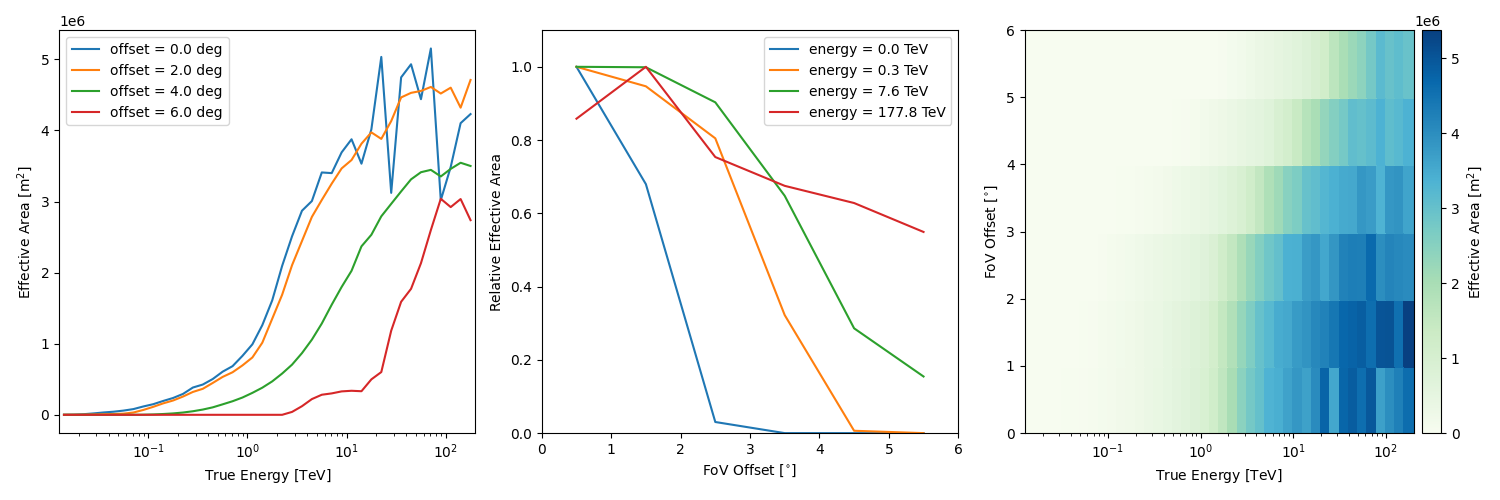
aeff = EffectiveAreaTable2D.read(irf_filename, hdu="EFFECTIVE AREA")
print(aeff)
EffectiveAreaTable2D
--------------------

  axes  : ['energy_true', 'offset']
  shape : (42, 6)
  ndim  : 2
  unit  : m2
  dtype : >f4
We can see that the Effective Area Table is defined in terms of
energy_true and offset from the camera center
MapAxis

        name       : offset
        unit       : 'deg'
        nbins      : 6
        node type  : edges
        edges min  : 0.0e+00 deg
        edges max  : 6.0e+00 deg
        interp     : lin

[[3.9391360e+02 2.6772235e+02 1.1955810e+01 0.0000000e+00 0.0000000e+00
  0.0000000e+00]
 [2.1976572e+03 1.3710784e+03 6.6018166e+01 0.0000000e+00 0.0000000e+00
  0.0000000e+00]
 [7.2827988e+03 4.4933657e+03 1.9277492e+02 0.0000000e+00 0.0000000e+00
  0.0000000e+00]
 [1.6318811e+04 9.2217412e+03 3.9053906e+02 0.0000000e+00 0.0000000e+00
  0.0000000e+00]
 [2.7097381e+04 1.5188338e+04 7.1269263e+02 0.0000000e+00 0.0000000e+00
  0.0000000e+00]
 [3.5835918e+04 2.0376213e+04 1.4120719e+03 6.4971704e+00 0.0000000e+00
  0.0000000e+00]
 [4.8613613e+04 2.7351418e+04 4.6046689e+03 8.7537086e+01 0.0000000e+00
  0.0000000e+00]
 [6.8954039e+04 4.6218742e+04 1.8455480e+04 7.0139252e+02 0.0000000e+00
  0.0000000e+00]
 [1.0631757e+05 8.4360750e+04 5.2121164e+04 3.4875723e+03 0.0000000e+00
  0.0000000e+00]
 [1.4225631e+05 1.2825456e+05 9.6194453e+04 1.0149044e+04 0.0000000e+00
  0.0000000e+00]
 [1.8893600e+05 1.7755386e+05 1.4428634e+05 2.2362506e+04 6.2068682e+00
  0.0000000e+00]
 [2.3058422e+05 2.1899070e+05 1.8349780e+05 3.8943121e+04 1.1567629e+01
  0.0000000e+00]
 [2.8908866e+05 2.7990194e+05 2.3380311e+05 6.3812160e+04 1.5692809e+02
  0.0000000e+00]
 [3.7190994e+05 3.4834488e+05 2.9489822e+05 9.9163195e+04 8.5162628e+02
  5.3302565e+00]
 [4.1554106e+05 3.9529719e+05 3.3659253e+05 1.4420073e+05 3.4303606e+03
  0.0000000e+00]
 [4.9977859e+05 4.9269494e+05 4.0322775e+05 1.9834338e+05 1.1456479e+04
  0.0000000e+00]
 [5.9969731e+05 5.8570719e+05 4.8037638e+05 2.6652219e+05 2.7997221e+04
  3.0902437e+01]
 [6.7681656e+05 6.6181862e+05 5.3499075e+05 3.2443672e+05 5.7385727e+04
  1.8062607e+02]
 [8.1099306e+05 7.7395744e+05 6.1618850e+05 3.8555500e+05 1.0076540e+05
  9.7876233e+02]
 [9.5867488e+05 8.9280475e+05 7.2040469e+05 4.5892966e+05 1.5842497e+05
  4.7765957e+03]
 [1.2162670e+06 1.1264500e+06 9.0183519e+05 5.3590188e+05 2.2699878e+05
  1.5607778e+04]
 [1.5719922e+06 1.4968236e+06 1.2062580e+06 6.4819444e+05 2.9215375e+05
  5.0505949e+04]
 [2.0122385e+06 1.8475576e+06 1.5297030e+06 7.8799800e+05 3.7284447e+05
  1.0520119e+05]
 [2.4420222e+06 2.3037632e+06 1.9053655e+06 9.5194769e+05 4.5951631e+05
  1.8031431e+05]
 [2.7887840e+06 2.6253652e+06 2.2635108e+06 1.2041222e+06 5.3117988e+05
  2.5779092e+05]
 [3.0016288e+06 2.9912648e+06 2.5768262e+06 1.5230376e+06 5.9205875e+05
  3.4480056e+05]
 [3.3368855e+06 3.1926520e+06 2.8515948e+06 1.8699165e+06 6.9847406e+05
  4.2104353e+05]
 [3.4212028e+06 3.4642048e+06 3.0395135e+06 2.1510240e+06 9.4647544e+05
  5.1629219e+05]
 [3.6419578e+06 3.5427520e+06 3.3886270e+06 2.4904078e+06 1.1061971e+06
  5.8834862e+05]
 [3.8369650e+06 3.7596682e+06 3.4080942e+06 2.6554088e+06 1.3962942e+06
  6.9074812e+05]
 [3.6556248e+06 3.9023670e+06 3.7240965e+06 2.9912712e+06 1.7479085e+06
  8.0375512e+05]
 [4.0462798e+06 4.1072542e+06 3.8377268e+06 3.0739282e+06 1.9910796e+06
  9.9608912e+05]
 [4.7580410e+06 4.2058705e+06 3.5561760e+06 3.2560538e+06 2.3279955e+06
  1.1768896e+06]
 [3.5545130e+06 4.4198250e+06 3.8441040e+06 3.3812120e+06 2.5538942e+06
  1.6402822e+06]
 [4.7350380e+06 4.7123895e+06 4.2164425e+06 3.5192420e+06 2.7652512e+06
  1.9816452e+06]
 [4.8769240e+06 4.7692170e+06 4.2880470e+06 3.5438860e+06 3.0800792e+06
  2.2079930e+06]
 [4.5754970e+06 4.8475650e+06 4.2628525e+06 3.8222980e+06 3.0025508e+06
  2.4225498e+06]
 [4.9606540e+06 4.5763635e+06 4.6471115e+06 3.7471700e+06 3.1438465e+06
  2.7804888e+06]
 [3.6909290e+06 5.0354700e+06 4.0028272e+06 3.3364130e+06 3.3689322e+06
  3.1486415e+06]
 [4.0064830e+06 5.0474750e+06 4.1556008e+06 3.8290458e+06 3.0894640e+06
  2.9776920e+06]
 [4.2465055e+06 4.5345275e+06 4.1062535e+06 3.8885138e+06 3.2021345e+06
  3.0907128e+06]
 [4.6105760e+06 5.3715810e+06 4.0482342e+06 3.6259962e+06 3.3739292e+06
  2.9499210e+06]]
[ 900269.83242471 3398360.62514628] m2
Similarly, we can access other IRFs as well
psf = EnergyDependentMultiGaussPSF.read(irf_filename, hdu="Point Spread Function")
bkg = Background3D.read(irf_filename, hdu="BACKGROUND")
edisp = EnergyDispersion2D.read(irf_filename, hdu="ENERGY DISPERSION")

print(bkg)
Background3D
------------

  axes  : ['energy', 'fov_lon', 'fov_lat']
  shape : (21, 36, 36)
  ndim  : 3
  unit  : 1 / (MeV s sr)
  dtype : >f4
Note that the background is given in FoV coordinates with fov_lon
and fov_lat axis, and not in offset from the camera center. We
can also check the Field of view alignment. Currently, two possible
alignments are supported: alignment with the horizontal coordinate
system (ALTAZ) and alignment with the equatorial coordinate system
(RADEC).
print(bkg.fov_alignment)
FoVAlignment.RADEC
To evaluate the IRFs, pass the values for each axis. To know the default interpolation scheme for the data
print(bkg.interp_kwargs)

# Evaluate background
# Note that evaluate functions support  numpy-style broadcasting
energy = [1, 10, 100, 1000] * u.TeV
fov_lon = [1, 2] * u.deg
fov_lat = [1, 2] * u.deg
ev = bkg.evaluate(
    energy=energy.reshape(-1, 1, 1),
    fov_lat=fov_lat.reshape(1, -1, 1),
    fov_lon=fov_lon.reshape(1, 1, -1),
)
print(ev)
{'bounds_error': False, 'fill_value': 0.0, 'values_scale': 'log'}
[[[1.27093776e-04 1.12423250e-04]
  [1.12423250e-04 9.85188496e-05]]

 [[7.67759236e-07 9.01235137e-07]
  [9.01235137e-07 1.05901956e-06]]

 [[5.74465974e-09 5.24685677e-09]
  [5.24685677e-09 4.65357608e-09]]

 [[0.00000000e+00 0.00000000e+00]
  [0.00000000e+00 0.00000000e+00]]] 1 / (MeV s sr)
We can customise the interpolation scheme. Here, we adapt to fill
nan instead of 0 for extrapolated values
[[[1.27093776e-04 1.12423250e-04]
  [1.12423250e-04 9.85188496e-05]]

 [[7.67759236e-07 9.01235137e-07]
  [9.01235137e-07 1.05901956e-06]]

 [[5.74465974e-09 5.24685677e-09]
  [5.24685677e-09 4.65357608e-09]]

 [[           nan            nan]
  [           nan            nan]]] 1 / (MeV s sr)
The interpolation scheme along each axis is taken from the MapAxis
specification. eg
print(
"Interpolation scheme for energy axis is: ",
bkg.axes["energy"].interp,
"and for the fov_lon axis is: ",
bkg.axes["fov_lon"].interp,
)
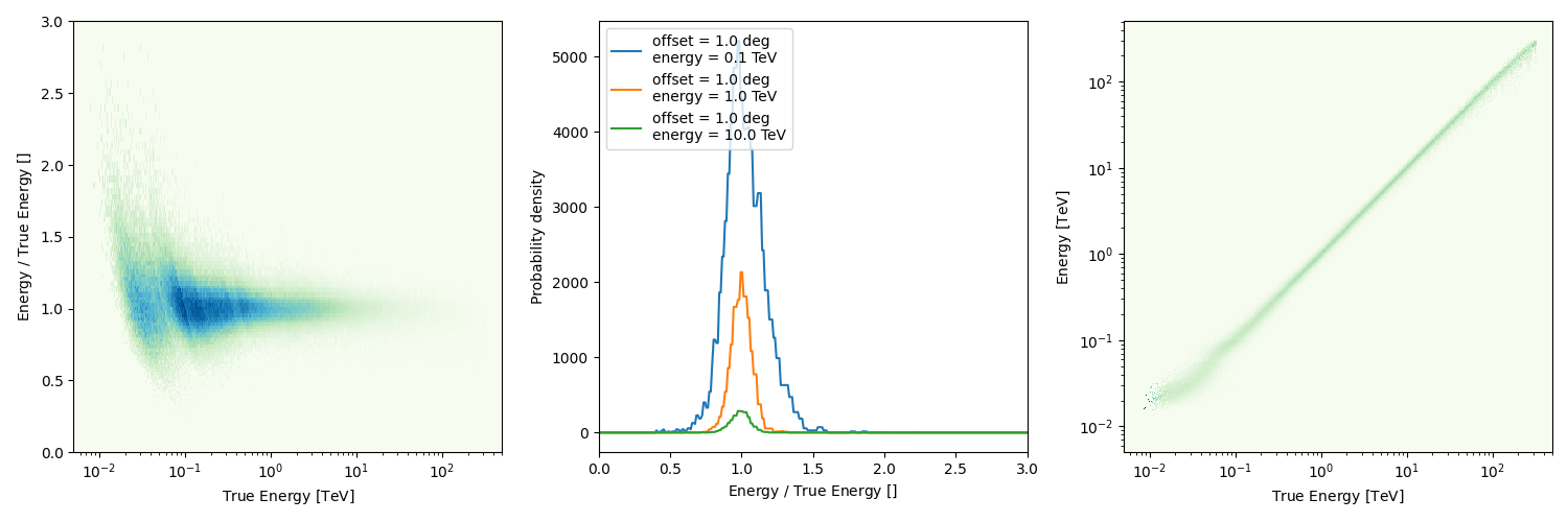
# Evaluate energy dispersion
ev = edisp.evaluate(energy_true=1 * u.TeV, offset=[0, 1] * u.deg, migra=[1, 1.2])
print(ev)
edisp.peek()
print(psf)
Interpolation scheme for energy axis is:  log and for the fov_lon axis is:  lin
[189.80982039  54.28382603]
EnergyDependentMultiGaussPSF
----------------------------

  axes      : ['energy_true', 'offset']
  shape     : (25, 6)
  ndim      : 2
  parameters: ['sigma_1', 'sigma_2', 'sigma_3', 'scale', 'ampl_2', 'ampl_3']
The PointSpreadFunction for the CTA DC1 is stored as a combination of 3
Gaussians. Other PSFs, like a PSF_TABLE and analytic expressions
like KING function are also supported. All PSF classes inherit from a
common base PSF class.
print(psf.axes.names)

# To get the containment radius for a fixed fraction at a given position
print(
    psf.containment_radius(
        fraction=0.68, energy_true=1.0 * u.TeV, offset=[0.2, 4.0] * u.deg
    )
)

# Alternatively, to get the containment fraction for at a given position
print(
    psf.containment(
        rad=0.05 * u.deg, energy_true=1.0 * u.TeV, offset=[0.2, 4.0] * u.deg
    )
)
['energy_true', 'offset']
[0.05075 0.08075] deg
[0.66984341 0.35569283]
Support for Asymmetric IRFs#
While Gammapy does not have inbuilt classes for supporting asymmetric
IRFs (except for Background3D), custom classes can be created. For
this to work correctly with the MapDatasetMaker, only variations
with fov_lon and fov_lat can be allowed.
The main idea is that the list of required axes should be correctly mentioned in the class definition.
Effective Area#
class EffectiveArea3D(IRF):
tag = "aeff_3d"
required_axes = ["energy_true", "fov_lon", "fov_lat"]
default_unit = u.m**2
energy_axis = MapAxis.from_energy_edges(
[0.1, 0.3, 1.0, 3.0, 10.0] * u.TeV, name="energy_true"
)
nbin = 7
fov_lon_axis = MapAxis.from_edges([-1.5, -0.5, 0.5, 1.5] * u.deg, name="fov_lon")
fov_lat_axis = MapAxis.from_edges([-1.5, -0.5, 0.5, 1.5] * u.deg, name="fov_lat")
data = np.ones((4, 3, 3))
for i in range(1, 4):
data[i] = data[i - 1] * 2.0
data[i][-1] = data[i][0] * 1.2
aeff_3d = EffectiveArea3D(
[energy_axis, fov_lon_axis, fov_lat_axis], data=data, unit=u.m**2
)
print(aeff_3d)
res = aeff_3d.evaluate(
fov_lon=[-0.5, 0.8] * u.deg,
fov_lat=[-0.5, 1.0] * u.deg,
energy_true=[0.2, 8.0] * u.TeV,
)
print(res)
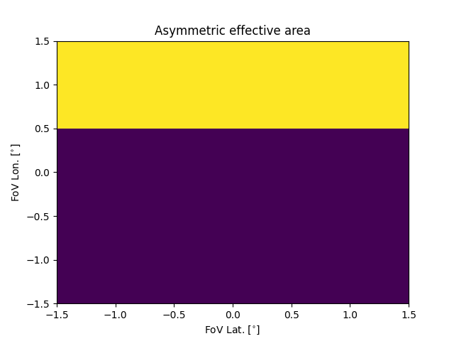
# to visualise at a given energy
aeff_eval = aeff_3d.evaluate(energy_true=[1.0] * u.TeV)
ax = plt.subplot()
with quantity_support():
caxes = ax.pcolormesh(
fov_lat_axis.edges, fov_lon_axis.edges, aeff_eval.value.squeeze()
)
fov_lat_axis.format_plot_xaxis(ax)
fov_lon_axis.format_plot_yaxis(ax)
ax.set_title("Asymmetric effective area")
EffectiveArea3D
---------------

  axes  : ['energy_true', 'fov_lon', 'fov_lat']
  shape : (4, 3, 3)
  ndim  : 3
  unit  : m2
  dtype : float64

[ 1.12493874 10.80683246] m2

Text(0.5, 1.0, 'Asymmetric effective area')
Unless specified, it is assumed these IRFs are in the RADEC frame
<FoVAlignment.RADEC: 'RADEC'>
Serialisation#
For serialisation, we need to add the class definition to the
IRF_DL3_HDU_SPECIFICATION dictionary
IRF_DL3_HDU_SPECIFICATION["aeff_3d"] = {
    "extname": "EFFECTIVE AREA",
    "column_name": "EFFAREA",
    "mandatory_keywords": {
        **COMMON_IRF_HEADERS,
        "HDUCLAS2": "EFF_AREA",
        "HDUCLAS3": "FULL-ENCLOSURE",  # added here to have HDUCLASN in order
        "HDUCLAS4": "AEFF_3D",
    },
}

aeff_3d.write("test_aeff3d.fits", overwrite=True)

aeff_new = EffectiveArea3D.read("test_aeff3d.fits")
print(aeff_new)
EffectiveArea3D
---------------

  axes  : ['energy_true', 'fov_lon', 'fov_lat']
  shape : (4, 3, 3)
  ndim  : 3
  unit  : m2
  dtype : >f8
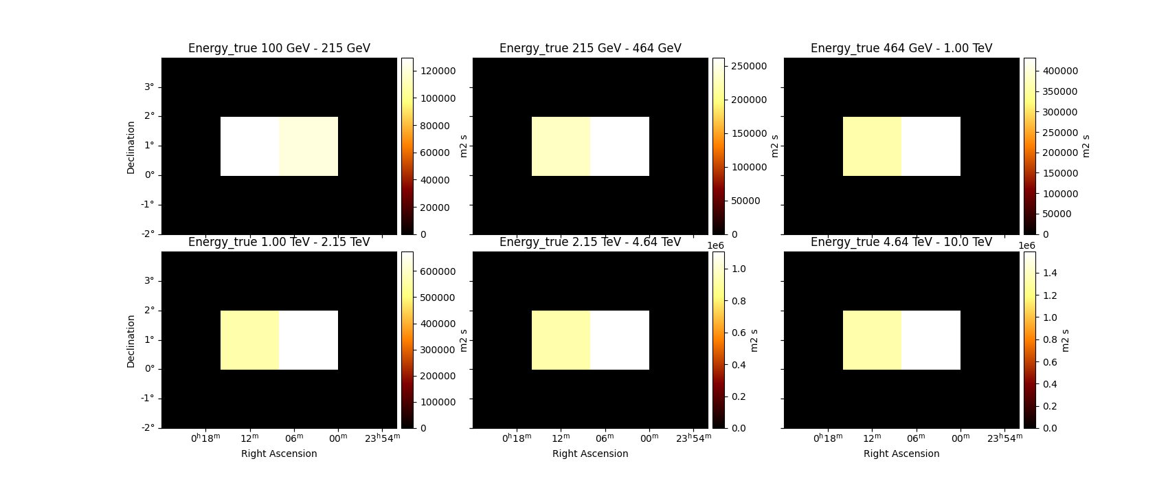
Create exposure map (DL4 product)#
DL4 data products can be created from these IRFs.
axis = MapAxis.from_energy_bounds(0.1 * u.TeV, 10 * u.TeV, 6, name="energy_true")
pointing = SkyCoord(2, 1, unit="deg")
geom = WcsGeom.create(npix=(4, 3), binsz=2, axes=[axis], skydir=pointing)

print(geom)

exposure_map = make_map_exposure_true_energy(
    pointing=pointing, livetime="42 h", aeff=aeff_3d, geom=geom
)

exposure_map.plot_grid(add_cbar=True, figsize=(17, 7))
plt.show()
WcsGeom

        axes       : ['lon', 'lat', 'energy_true']
        shape      : (4, 3, 6)
        ndim       : 3
        frame      : icrs
        projection : CAR
        center     : 2.0 deg, 1.0 deg
        width      : 8.0 deg x 6.0 deg
        wcs ref    : 2.0 deg, 1.0 deg
Energy Dispersion#
Note that most functions defined on the inbuilt IRF classes can be easily generalised to higher dimensions.
# Make a test case
energy_axis_true = MapAxis.from_energy_bounds(
    "0.1 TeV", "100 TeV", nbin=3, name="energy_true"
)

migra_axis = MapAxis.from_bounds(0, 4, nbin=2, node_type="edges", name="migra")

fov_lon_axis = MapAxis.from_edges([-1.5, -0.5, 0.5, 1.5] * u.deg, name="fov_lon")
fov_lat_axis = MapAxis.from_edges([-1.5, -0.5, 0.5, 1.5] * u.deg, name="fov_lat")

data = np.array(
    [
        [
            [
                [5.00e-01, 5.10e-01, 5.20e-01],
                [6.00e-01, 6.10e-01, 6.30e-01],
                [6.00e-01, 6.00e-01, 6.00e-01],
            ],
            [
                [2.0e-02, 2.0e-02, 2.0e-03],
                [2.0e-02, 2.0e-02, 2.0e-03],
                [2.0e-02, 2.0e-02, 2.0e-03],
            ],
        ],
        [
            [
                [5.00e-01, 5.10e-01, 5.20e-01],
                [6.00e-01, 6.10e-01, 6.30e-01],
                [6.00e-01, 6.00e-01, 6.00e-01],
            ],
            [
                [3.0e-02, 6.0e-02, 2.0e-03],
                [3.0e-02, 5.0e-02, 2.0e-03],
                [3.0e-02, 4.0e-02, 2.0e-03],
            ],
        ],
    ]
)


edisp3d = EnergyDispersion3D(
    [energy_axis_true, migra_axis, fov_lon_axis, fov_lat_axis], data=data
)

print(edisp3d)

energy = [1, 2] * u.TeV
migra = np.array([0.98, 0.97, 0.7])
fov_lon = [0.1, 1.5] * u.deg
fov_lat = [0.0, 0.3] * u.deg

edisp_eval = edisp3d.evaluate(
    energy_true=energy.reshape(-1, 1, 1, 1),
    migra=migra.reshape(1, -1, 1, 1),
    fov_lon=fov_lon.reshape(1, 1, -1, 1),
    fov_lat=fov_lat.reshape(1, 1, 1, -1),
)
print(edisp_eval[0])
EnergyDispersion3D
------------------

  axes  : ['energy_true', 'migra', 'fov_lon', 'fov_lat']
  shape : (3, 2, 3, 3)
  ndim  : 4
  unit  :
  dtype : float64

[[[0.61489  0.620398]
  [0.60075  0.597774]]

 [[0.617835 0.623397]
  [0.603625 0.600661]]

 [[0.69735  0.70437 ]
  [0.68125  0.67861 ]]]
Serialisation#
IRF_DL3_HDU_SPECIFICATION["edisp_3d"] = {
    "extname": "ENERGY DISPERSION",
    "column_name": "MATRIX",
    "mandatory_keywords": {
        **COMMON_IRF_HEADERS,
        "HDUCLAS2": "EDISP",
        "HDUCLAS3": "FULL-ENCLOSURE",  # added here to have HDUCLASN in order
        "HDUCLAS4": "EDISP_3D",
    },
}

edisp3d.write("test_edisp.fits", overwrite=True)

edisp_new = EnergyDispersion3D.read("test_edisp.fits")
edisp_new
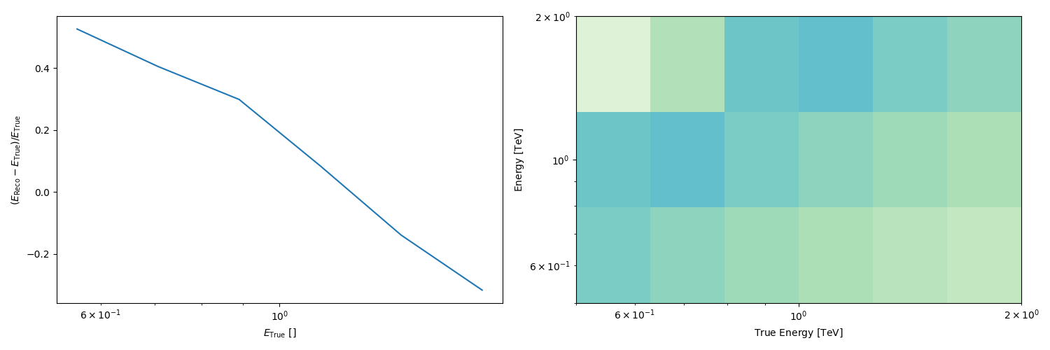
Create edisp kernel map (DL4 product) - EDispKernelMap#
migra = MapAxis.from_edges(np.linspace(0.5, 1.5, 50), unit="", name="migra")
etrue = MapAxis.from_energy_bounds(0.5, 2, 6, unit="TeV", name="energy_true")
ereco = MapAxis.from_energy_bounds(0.5, 2, 3, unit="TeV", name="energy")
geom = WcsGeom.create(10, binsz=0.5, axes=[ereco, etrue], skydir=pointing)

edispmap = make_edisp_kernel_map(edisp3d, pointing, geom)

edispmap.peek()
plt.show()

#
print(edispmap.edisp_map.data[3][1][3])
[0.         0.         0.19932878 0.20009124 0.20072608 0.20099855
 0.2009851  0.20097159 0.         0.        ]
PSF#
There are two types of asymmetric PSFs that can be considered:
asymmetry about the camera center: such PSF Tables can be supported,
asymmetry about the source position: these PSF models cannot be supported correctly within the data reduction scheme at present
Also, analytic PSF models defined within the GADF scheme cannot be directly generalised to the 3D case for use within Gammapy.
class PSF_assym(IRF):
    tag = "psf_assym"
    required_axes = ["energy_true", "fov_lon", "fov_lat", "rad"]
    default_unit = u.sr**-1


energy_axis = MapAxis.from_energy_edges(
    [0.1, 0.3, 1.0, 3.0, 10.0] * u.TeV, name="energy_true"
)

nbin = 7
fov_lon_axis = MapAxis.from_edges([-1.5, -0.5, 0.5, 1.5] * u.deg, name="fov_lon")
fov_lat_axis = MapAxis.from_edges([-1.5, -0.5, 0.5, 1.5] * u.deg, name="fov_lat")

rad_axis = MapAxis.from_edges([0, 1, 2], unit="deg", name="rad")

data = 0.1 * np.ones((4, 3, 3, 2))
for i in range(1, 4):
    data[i] = data[i - 1] * 1.5


psf_assym = PSF_assym(
    axes=[energy_axis, fov_lon_axis, fov_lat_axis, rad_axis],
    data=data,
)
print(psf_assym)

energy = [1, 2] * u.TeV
rad = np.array([0.98, 0.97, 0.7]) * u.deg
fov_lon = [0.1, 1.5] * u.deg
fov_lat = [0.0, 0.3] * u.deg

psf_assym.evaluate(
    energy_true=energy.reshape(-1, 1, 1, 1),
    rad=rad.reshape(1, -1, 1, 1),
    fov_lon=fov_lon.reshape(1, 1, -1, 1),
    fov_lat=fov_lat.reshape(1, 1, 1, -1),
)
PSF_assym
---------

  axes  : ['energy_true', 'fov_lon', 'fov_lat', 'rad']
  shape : (4, 3, 3, 2)
  ndim  : 4
  unit  :
  dtype : float64


<Quantity [[[[0.18921591, 0.18921591],
             [0.18921591, 0.18921591]],

            [[0.18921591, 0.18921591],
             [0.18921591, 0.18921591]],

            [[0.18921591, 0.18921591],
             [0.18921591, 0.18921591]]],


           [[[0.23905561, 0.23905561],
             [0.23905561, 0.23905561]],

            [[0.23905561, 0.23905561],
             [0.23905561, 0.23905561]],

            [[0.23905561, 0.23905561],
             [0.23905561, 0.23905561]]]]>
Serialisation#
IRF_DL3_HDU_SPECIFICATION["psf_assym"] = {
    "extname": "POINT SPREAD FUNCTION",
    "column_name": "MATRIX",
    "mandatory_keywords": {
        **COMMON_IRF_HEADERS,
        "HDUCLAS2": "PSF",
        "HDUCLAS3": "FULL-ENCLOSURE",
        "HDUCLAS4": "PSFnD",
    },
}

psf_assym.write("test_psf.fits.gz", overwrite=True)

psf_new = PSF_assym.read("test_psf.fits.gz")
Create DL4 product - PSFMap#
rad = MapAxis.from_edges(np.linspace(0.5, 3.0, 10), unit="deg", name="rad")
etrue = MapAxis.from_energy_bounds(0.5, 2, 6, unit="TeV", name="energy_true")
geom = WcsGeom.create(10, binsz=0.5, axes=[rad, etrue], skydir=pointing)

psfmap = make_psf_map(psf_assym, pointing, geom)

psfmap.peek()
plt.show()
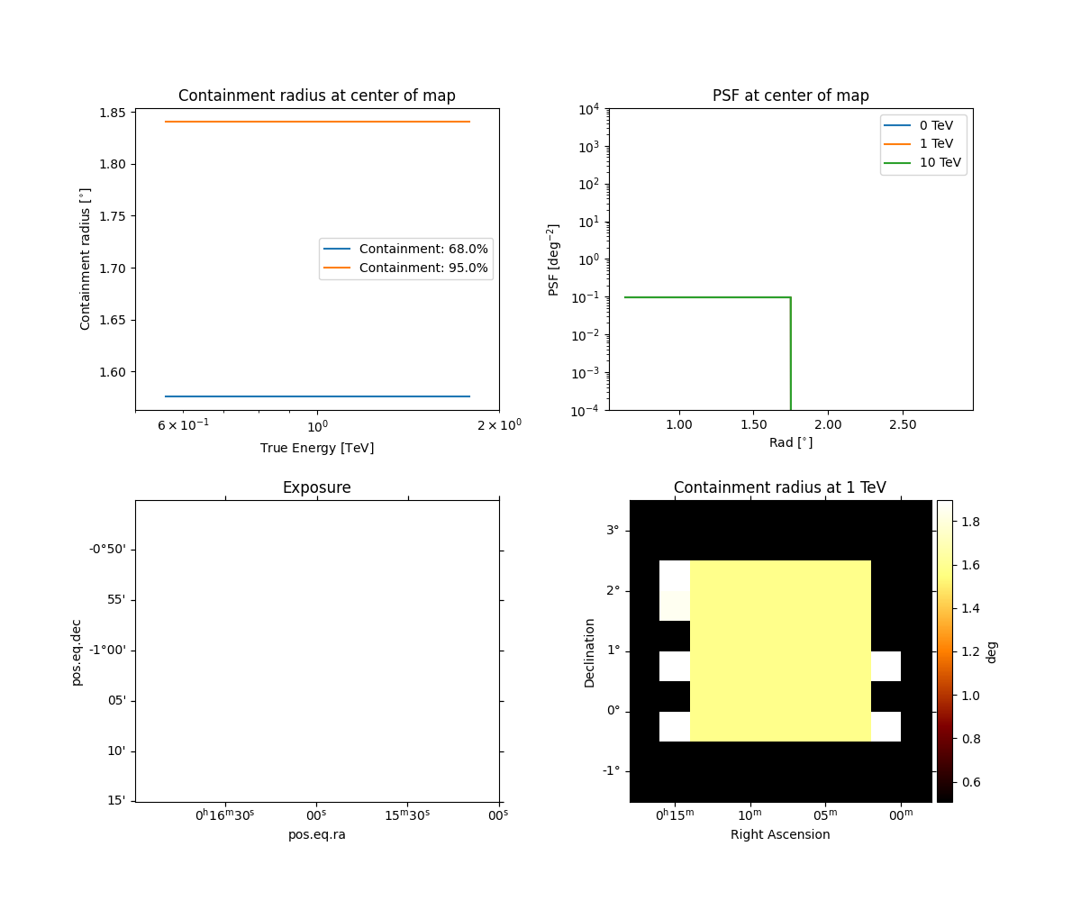
Containers for asymmetric analytic PSFs are not supported at present.
NOTE: Support for asymmetric IRFs is preliminary at the moment, and will evolve depending on feedback.