Note

Go to the end to download the full example code or to run this example in your browser via Binder

Observational clustering#

Clustering observations into specific groups.

Context#

Typically, observations from gamma-ray telescopes can span a number of different observation periods, therefore it is likely that the observation conditions and quality are not always the same. This tutorial aims to provide a way in which observations can be grouped such that similar observations are grouped together, and then the data reduction is performed.

Objective#

To cluster similar observations based on various quantities.

Proposed approach#

For completeness two different methods for grouping of observations are shown here.

A simple grouping based on zenith angle from an existing observations table.
Grouping the observations depending on the IRF quality, by means of hierarchical clustering.

import numpy as np
import astropy.units as u
from astropy.coordinates import SkyCoord
import matplotlib.pyplot as plt
from gammapy.data import DataStore
from gammapy.data.observations import Observations
from gammapy.data.utils import get_irfs_features
from gammapy.utils.cluster import hierarchical_clustering, standard_scaler

Obtain the observations#

First need to define the DataStore object for the HESS DL3 DR1 data. Next, utilise a cone search to select only the observations of interest. In this case, we choose PKS 2155-304 as the object of interest.

The ObservationTable is then filtered using the select_observations tool.

data_store = DataStore.from_dir("$GAMMAPY_DATA/hess-dl3-dr1")

selection = dict(
    type="sky_circle",
    frame="icrs",
    lon="329.71693826 deg",
    lat="-30.2255 deg",
    radius="2 deg",
)
obs_table = data_store.obs_table
selected_obs_table = obs_table.select_observations(selection)

More complex selection can be done by utilising the obs_table entries directly. We can now retrieve the relevant observations by passing their obs_id to the get_observations method.

obs_ids = selected_obs_table["OBS_ID"]
observations = data_store.get_observations(obs_ids)

Show various observation quantities#

Print here the range of zenith angles and muon efficiencies, to see if there is a sensible way to group the observations.

obs_zenith = selected_obs_table["ZEN_PNT"].to(u.deg)
obs_muoneff = selected_obs_table["MUONEFF"]

print(f"{np.min(obs_zenith):.2f} < zenith angle < {np.max(obs_zenith):.2f}")
print(f"{np.min(obs_muoneff):.2f} < muon efficiency < {np.max(obs_muoneff):.2f}")

7.23 deg < zenith angle < 50.42 deg
0.97 < muon efficiency < 1.03

Manual grouping of observations#

Here we can plot the zenith angle vs muon efficiency of the observations. We decide to group the observations according to their zenith angle. This is done manually as per a user defined cut, in this case we take the median value of the zenith angles to define each observation group.

This type of grouping can be utilised according to different parameters i.e. zenith angle, muon efficiency, offset angle. The quantity chosen can therefore be adjusted according to each specific science case.

median_zenith = np.median(obs_zenith)

labels = []
for obs in observations:
    zenith = obs.get_pointing_altaz(time=obs.tmid).zen
    labels.append("low_zenith" if zenith < median_zenith else "high_zenith")
grouped_observations = observations.group_by_label(labels)

print(grouped_observations)

{'group_high_zenith': <gammapy.data.observations.Observations object at 0x7f3bc1ab4cd0>, 'group_low_zenith': <gammapy.data.observations.Observations object at 0x7f3bc1ab4340>}

The results for each group of observations is shown visually below.

fix, ax = plt.subplots(1, 1, figsize=(7, 5))
for obs in grouped_observations["group_low_zenith"]:
    ax.plot(
        obs.get_pointing_altaz(time=obs.tmid).zen,
        obs.meta.optional["MUONEFF"],
        "d",
        color="red",
    )
for obs in grouped_observations["group_high_zenith"]:
    ax.plot(
        obs.get_pointing_altaz(time=obs.tmid).zen,
        obs.meta.optional["MUONEFF"],
        "o",
        color="blue",
    )
ax.set_ylabel("Muon efficiency")
ax.set_xlabel("Zenith angle (deg)")
ax.axvline(median_zenith.value, ls="--", color="black")
plt.show()

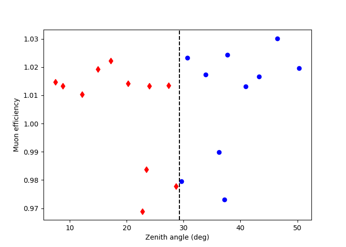
This shows the observations grouped by zenith angle. The diamonds are observations which have a zenith angle less than the median value, whilst the circles are observations above the median.

The grouped_observations provide a list of Observations which can be utilised in the usual way to show the various properties of the observations i.e. see the CTA with Gammapy tutorial.

Hierarchical clustering of observations#

This method shows how to cluster observations based on their IRF quantities, in this case those that have a similar edisp and psf. The get_irfs_features is utilised to achieve this. The observations are then clustered based on these criteria using hierarchical_clustering. The idea here is to minimise the variance of both edisp and psf within a specific group to limit the error on the quantity when they are stacked at the dataset level.

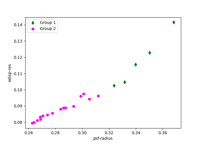
In this example, the irf features are computed for the edisp-res and psf-radius at 1 TeV. This is stored as a Table, as shown below.

source_position = SkyCoord(329.71693826 * u.deg, -30.2255890 * u.deg, frame="icrs")
names = ["edisp-res", "psf-radius"]
features_irfs = get_irfs_features(
    observations, energy_true="1 TeV", position=source_position, names=names
)
print(features_irfs)

     edisp-res      obs_id      psf-radius
                                   deg
------------------- ------ -------------------
36834038301420274  33787 0.14149953611195087
339835555384604  33788 0.11553325504064559
3237948931463171  33789 0.10262943822890519
30535345877453707  33790 0.09426693227142095
28755283551095173  33791 0.08894569035619496
27409496735322464  33792 0.08447355125099419
26665050077722524  33793  0.0811551760882139
26272868097919794  33794 0.07943648658692837
2639554729438709  33795  0.0799109224230051
26887783978974283  33796 0.08191603310406206
2777074437073429  33797  0.0855013383552432
29355238360800506  33798  0.0897868126630783
31186857659616535  33799 0.09623312838375568
33164865722698683  33800 0.10470702368766069
3503706026275275  33801 0.12276676166802643
3011061699260256  47802 0.09740295372903346
2861432787940619  47803 0.08880368117243051
27057337686547633  47804 0.08388624433428049
29882214027996945  47827 0.09610314778983592
28385358839966657  47828 0.08795162606984375
268663733018811  47829 0.08328557573258877

Compute standardized features by removing the mean and scaling to unit variance:

scaled_features_irfs = standard_scaler(features_irfs)
print(scaled_features_irfs)

     edisp-res       obs_id       psf-radius
-------------------- ------ ---------------------
  2.3885947175689592  33787     3.053212009682775
  1.4351637481047363  33788     1.363472509034498
  0.8986348363207728  33789    0.5237647004325865
  0.2818047723094509  33790 -0.020420144596410953
 -0.3135914081482271  33791  -0.36669663417038234
 -0.7637308880733709  33792   -0.6577182894355391
  -1.012733796525585  33793    -0.873659477745188
 -1.1439110308062257  33794    -0.985502122122975
  -1.102877228833871  33795   -0.9546285068162436
 -0.9382336444241555  33796   -0.8241471833009617
 -0.6429005895278312  33797    -0.590835686434463
-0.11291820875721864  33798   -0.3119611261122878
 0.49972277488662115  33799   0.10752883769757363
  1.1613279491744304  33800    0.6589622747787678
  1.7875405607868806  33801    1.8341884287660133
  0.1397412321592923  47802    0.1836544903987521
-0.36073833513766157  47803   -0.3759377929871826
 -0.8815212313941426  47804   -0.6959369197218669
 0.06334488877417636  47827   0.09907043184188653
 -0.4373240195300975  47828   -0.4313847458879893
 -0.9453950989269149  47829   -0.7350250533013533

The hierarchical_clustering then clusters this table into t=2 groups with a corresponding label for each group. In this case, we choose to cluster the observations into two groups. We can print this table to show the corresponding label which has been added to the previous feature_irfs table.

The arguments for fcluster are passed as a dictionary here.

features = hierarchical_clustering(scaled_features_irfs, fcluster_kwargs={"t": 2})
print(features)

     edisp-res       obs_id       psf-radius      labels
-------------------- ------ --------------------- ------
  2.3885947175689592  33787     3.053212009682775      1
  1.4351637481047363  33788     1.363472509034498      1
  0.8986348363207728  33789    0.5237647004325865      1
  0.2818047723094509  33790 -0.020420144596410953      2
 -0.3135914081482271  33791  -0.36669663417038234      2
 -0.7637308880733709  33792   -0.6577182894355391      2
  -1.012733796525585  33793    -0.873659477745188      2
 -1.1439110308062257  33794    -0.985502122122975      2
  -1.102877228833871  33795   -0.9546285068162436      2
 -0.9382336444241555  33796   -0.8241471833009617      2
 -0.6429005895278312  33797    -0.590835686434463      2
-0.11291820875721864  33798   -0.3119611261122878      2
 0.49972277488662115  33799   0.10752883769757363      2
  1.1613279491744304  33800    0.6589622747787678      1
  1.7875405607868806  33801    1.8341884287660133      1
  0.1397412321592923  47802    0.1836544903987521      2
-0.36073833513766157  47803   -0.3759377929871826      2
 -0.8815212313941426  47804   -0.6959369197218669      2
 0.06334488877417636  47827   0.09907043184188653      2
 -0.4373240195300975  47828   -0.4313847458879893      2
 -0.9453950989269149  47829   -0.7350250533013533      2

Finally, observations.group_by_label creates a dictionary containing t Observations objects by grouping the similar labels.

obs_clusters = observations.group_by_label(features["labels"])
print(obs_clusters)


mask_1 = features["labels"] == 1
mask_2 = features["labels"] == 2
fix, ax = plt.subplots(1, 1, figsize=(7, 5))
ax.set_ylabel("edisp-res")
ax.set_xlabel("psf-radius")
ax.plot(
    features_irfs[mask_1]["edisp-res"],
    features_irfs[mask_1]["psf-radius"],
    "d",
    color="green",
    label="Group 1",
)
ax.plot(
    features_irfs[mask_2]["edisp-res"],
    features_irfs[mask_2]["psf-radius"],
    "o",
    color="magenta",
    label="Group 2",
)
ax.legend()
plt.show()

{'group_1': <gammapy.data.observations.Observations object at 0x7f3be846ab80>, 'group_2': <gammapy.data.observations.Observations object at 0x7f3be846a3d0>}

The groups here are divided by the quality of the IRFs values edisp-res and psf-radius. The diamond and circular points indicate how the observations are grouped.

In both examples we have a set of Observation objects which can be reduced using the DatasetsMaker to create two (in this specific case) separate datasets. These can then be jointly fitted using the Multi instrument joint 3D and 1D analysis tutorial.

Gallery generated by Sphinx-Gallery