Note
Go to the end to download the full example code. or to run this example in your browser via Binder
Makers - Data reduction#
Data reduction: from observations to binned datasets
Introduction#
The gammapy.makers sub-package contains classes to perform data
reduction tasks from DL3 data to binned datasets. In the data reduction
step the DL3 data is prepared for modeling and fitting, by binning
events into a counts map and interpolating the exposure, background, psf
and energy dispersion on the chosen analysis geometry.
Setup#
import numpy as np
from astropy import units as u
from astropy.coordinates import SkyCoord
from regions import CircleSkyRegion
import matplotlib.pyplot as plt
from gammapy.data import DataStore
from gammapy.datasets import Datasets, MapDataset, SpectrumDataset
from gammapy.makers import (
    DatasetsMaker,
    FoVBackgroundMaker,
    MapDatasetMaker,
    ReflectedRegionsBackgroundMaker,
    SafeMaskMaker,
    SpectrumDatasetMaker,
)
from gammapy.makers.utils import make_effective_livetime_map, make_observation_time_map
from gammapy.maps import MapAxis, RegionGeom, WcsGeom
Check setup#
from gammapy.utils.check import check_tutorials_setup

check_tutorials_setup()
System:

        python_executable      : /home/runner/work/gammapy-docs/gammapy-docs/gammapy/.tox/build_docs/bin/python
        python_version         : 3.9.22
        machine                : x86_64
        system                 : Linux


Gammapy package:

        version                : 2.0.dev1224+g83b25692c
        path                   : /home/runner/work/gammapy-docs/gammapy-docs/gammapy/.tox/build_docs/lib/python3.9/site-packages/gammapy


Other packages:

        numpy                  : 1.26.4
        scipy                  : 1.13.1
        astropy                : 6.0.1
        regions                : 0.8
        click                  : 8.1.8
        yaml                   : 6.0.2
        IPython                : 8.18.1
        jupyterlab             : not installed
        matplotlib             : 3.9.4
        pandas                 : not installed
        healpy                 : 1.17.3
        iminuit                : 2.31.1
        sherpa                 : 4.16.1
        naima                  : 0.10.0
        emcee                  : 3.1.6
        corner                 : 2.2.3
        ray                    : 2.46.0


Gammapy environment variables:

        GAMMAPY_DATA           : /home/runner/work/gammapy-docs/gammapy-docs/gammapy-datasets/dev
Dataset#
The counts, exposure, background and IRF maps are bundled together in a
data structure named MapDataset.
The first step of the data reduction is to create an empty dataset. A
MapDataset can be created from any WcsGeom
object. This is illustrated in the following example:
energy_axis = MapAxis.from_bounds(
    1, 10, nbin=11, name="energy", unit="TeV", interp="log"
)
geom = WcsGeom.create(
    skydir=(83.63, 22.01),
    axes=[energy_axis],
    width=5 * u.deg,
    binsz=0.05 * u.deg,
    frame="icrs",
)
dataset_empty = MapDataset.create(geom=geom)
print(dataset_empty)
MapDataset
----------

  Name                            : yRUdUeoa

  Total counts                    : 0
  Total background counts         : 0.00
  Total excess counts             : 0.00

  Predicted counts                : 0.00
  Predicted background counts     : 0.00
  Predicted excess counts         : nan

  Exposure min                    : 0.00e+00 m2 s
  Exposure max                    : 0.00e+00 m2 s

  Number of total bins            : 110000
  Number of fit bins              : 0

  Fit statistic type              : cash
  Fit statistic value (-2 log(L)) : nan

  Number of models                : 0
  Number of parameters            : 0
  Number of free parameters       : 0
It is possible to compute the instrument response functions with different spatial and energy bins as compared to the counts and background maps. For example, one can specify a true energy axis which defines the energy binning of the IRFs:
energy_axis_true = MapAxis.from_bounds(
    0.3, 10, nbin=31, name="energy_true", unit="TeV", interp="log"
)
dataset_empty = MapDataset.create(geom=geom, energy_axis_true=energy_axis_true)
For the detail of the other options available, you can always call the help:
help(MapDataset.create)
Help on method create in module gammapy.datasets.map:

create(geom, energy_axis_true=None, migra_axis=None, rad_axis=None, binsz_irf=<Quantity 0.2 deg>, reference_time='2000-01-01', name=None, meta_table=None, reco_psf=False, **kwargs) method of abc.ABCMeta instance
    Create a MapDataset object with zero filled maps.

    Parameters
    ----------
    geom : `~gammapy.maps.WcsGeom`
        Reference target geometry in reco energy, used for counts and background maps.
    energy_axis_true : `~gammapy.maps.MapAxis`, optional
        True energy axis used for IRF maps. Default is None.
    migra_axis : `~gammapy.maps.MapAxis`, optional
        If set, this provides the migration axis for the energy dispersion map.
        If not set, an EDispKernelMap is produced instead. Default is None.
    rad_axis : `~gammapy.maps.MapAxis`, optional
        Rad axis for the PSF map. Default is None.
    binsz_irf : float
        IRF Map pixel size in degrees. Default is BINSZ_IRF_DEFAULT.
    reference_time : `~astropy.time.Time`
        The reference time to use in GTI definition. Default is "2000-01-01".
    name : str, optional
        Name of the returned dataset. Default is None.
    meta_table : `~astropy.table.Table`, optional
        Table listing information on observations used to create the dataset.
        One line per observation for stacked datasets. Default is None.
    reco_psf : bool
        Use reconstructed energy for the PSF geometry. Default is False.

    Returns
    -------
    empty_maps : `MapDataset`
        A MapDataset containing zero filled maps.

    Examples
    --------
    >>> from gammapy.datasets import MapDataset
    >>> from gammapy.maps import WcsGeom, MapAxis

    >>> energy_axis = MapAxis.from_energy_bounds(1.0, 10.0, 4, unit="TeV")
    >>> energy_axis_true = MapAxis.from_energy_bounds(
    ...            0.5, 20, 10, unit="TeV", name="energy_true"
    ...        )
    >>> geom = WcsGeom.create(
    ...            skydir=(83.633, 22.014),
    ...            binsz=0.02, width=(2, 2),
    ...            frame="icrs",
    ...            proj="CAR",
    ...            axes=[energy_axis]
    ...        )
    >>> empty = MapDataset.create(geom=geom, energy_axis_true=energy_axis_true, name="empty")
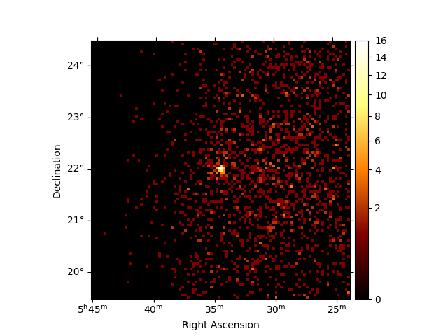
Once this empty “reference” dataset is defined, it can be filled with
observational data using the MapDatasetMaker:
# get observation
data_store = DataStore.from_dir("$GAMMAPY_DATA/hess-dl3-dr1")
obs = data_store.get_observations([23592])[0]

# fill dataset
maker = MapDatasetMaker()
dataset = maker.run(dataset_empty, obs)
print(dataset)

dataset.counts.sum_over_axes().plot(stretch="sqrt", add_cbar=True)
plt.show()
MapDataset
----------

  Name                            : Gy1V2-Q9

  Total counts                    : 2016
  Total background counts         : 1866.72
  Total excess counts             : 149.28

  Predicted counts                : 1866.72
  Predicted background counts     : 1866.72
  Predicted excess counts         : nan

  Exposure min                    : 1.19e+02 m2 s
  Exposure max                    : 1.09e+09 m2 s

  Number of total bins            : 110000
  Number of fit bins              : 110000

  Fit statistic type              : cash
  Fit statistic value (-2 log(L)) : nan

  Number of models                : 0
  Number of parameters            : 0
  Number of free parameters       : 0
The MapDatasetMaker fills the corresponding counts,
exposure, background, psf and edisp map per observation.
The MapDatasetMaker has a selection parameter, in case some of
the maps should not be computed. There is also a
background_oversampling parameter that defines the oversampling
factor in energy used to compute the background (default is None).
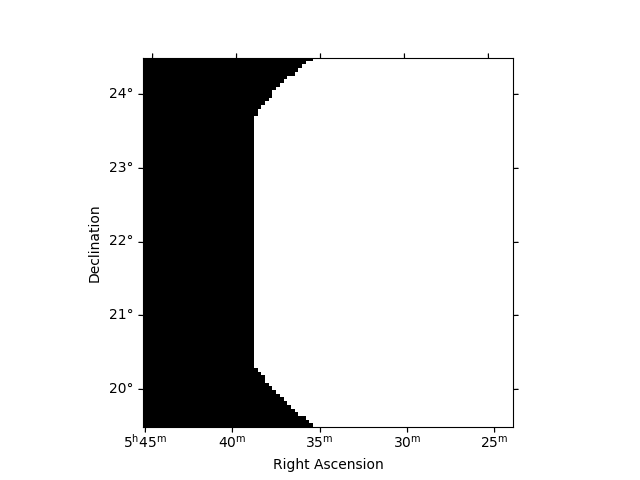
Safe data range handling#
To exclude the data range from a MapDataset, that is associated with
high systematics on instrument response functions, a mask_safe
can be defined. The mask_safe is a Map object
with bool data type, which indicates for each pixel, whether it should be included in
the analysis. The convention is that a value of True or 1
includes the pixel, while a value of False or 0 excludes a
pixels from the analysis. To compute safe data range masks according to
certain criteria, Gammapy provides a SafeMaskMaker class. The
different criteria are given by the methods argument, available
options are :
aeff-default, uses the energy ranged specified in the DL3 data files, if available.
aeff-max, the lower energy threshold is determined such as the effective area is above a given percentage of its maximum
edisp-bias, the lower energy threshold is determined such as the energy bias is below a given percentage
offset-max, the data beyond a given offset radius from the observation center are excluded
bkg-peak, the energy threshold is defined as the upper edge of the energy bin with the highest predicted background rate. This method was introduced in the H.E.S.S. DL3 validation paper
Note that currently some methods computing a safe energy range (“aeff-default”, “aeff-max” and “edisp-bias”) determine a true energy range and apply it to reconstructed energy, effectively neglecting the energy dispersion.
Multiple methods can be combined. Here is an example :
safe_mask_maker = SafeMaskMaker(
    methods=["aeff-default", "offset-max"], offset_max="3 deg"
)

dataset = maker.run(dataset_empty, obs)
dataset = safe_mask_maker.run(dataset, obs)
print(dataset.mask_safe)

dataset.mask_safe.sum_over_axes().plot()
plt.show()
WcsNDMap

        geom  : WcsGeom
        axes  : ['lon', 'lat', 'energy']
        shape : (100, 100, 11)
        ndim  : 3
        unit  :
        dtype : bool
The SafeMaskMaker does not modify any data, but only defines the
mask_safe attribute. This means that the safe data range
can be defined and modified in between the data reduction and stacking
and fitting. For a joint-likelihood analysis of multiple observations
the safe mask is applied to the counts and predicted number of counts
map during fitting. This correctly accounts for contributions
(spill-over) by the PSF from outside the field of view.
Background estimation#
The background computed by the MapDatasetMaker gives the number of
counts predicted by the background IRF of the observation. Because its
actual normalization, or even its spectral shape, might be poorly
constrained, it is necessary to correct it with the data themselves.
This is the role of background estimation Makers.
FoV background#
If the background energy dependent morphology is well reproduced by the
background model stored in the IRF, it might be that its normalization
is incorrect and that some spectral corrections are necessary. This is
made possible thanks to the FoVBackgroundMaker. This
technique is recommended in most 3D data reductions. For more details
and usage, see the FoV background.
Here we are going to use a FoVBackgroundMaker that
will rescale the background model to the data excluding the region where
a known source is present. For more details on the way to create
exclusion masks see the mask maps notebook.
circle = CircleSkyRegion(center=geom.center_skydir, radius=0.2 * u.deg)
exclusion_mask = geom.region_mask([circle], inside=False)

fov_bkg_maker = FoVBackgroundMaker(method="scale", exclusion_mask=exclusion_mask)
dataset = fov_bkg_maker.run(dataset)
Other backgrounds production methods available are listed below.
Ring background#
If the background model does not reproduce well the morphology, a
classical approach consists in applying local corrections by smoothing
the data with a ring kernel. This allows to build a set of OFF counts
taking into account the imperfect knowledge of the background. This is
implemented in the RingBackgroundMaker which
transforms the Dataset in a MapDatasetOnOff. This technique is
mostly used for imaging, and should not be applied for 3D modeling and
fitting.
For more details and usage, see Ring background
Reflected regions background#
In the absence of a solid background model, a classical technique in
Cherenkov astronomy for 1D spectral analysis is to estimate the
background in a number of OFF regions. When the background can be safely
estimated as radially symmetric w.r.t. the pointing direction, one can
apply the reflected regions background technique. This is implemented in
the ReflectedRegionsBackgroundMaker which transforms
a SpectrumDataset in a SpectrumDatasetOnOff.
This method is only used for 1D spectral analysis.
For more details and usage, see the Reflected background
Data reduction loop#
The data reduction steps can be combined in a single loop to run a full
data reduction chain. For this the MapDatasetMaker is run first and
the output dataset is the passed on to the next maker step. Finally, the
dataset per observation is stacked into a larger map.
data_store = DataStore.from_dir("$GAMMAPY_DATA/hess-dl3-dr1")
observations = data_store.get_observations([23523, 23592, 23526, 23559])

energy_axis = MapAxis.from_bounds(
    1, 10, nbin=11, name="energy", unit="TeV", interp="log"
)
geom = WcsGeom.create(skydir=(83.63, 22.01), axes=[energy_axis], width=5, binsz=0.02)

dataset_maker = MapDatasetMaker()
safe_mask_maker = SafeMaskMaker(
    methods=["aeff-default", "offset-max"], offset_max="3 deg"
)

stacked = MapDataset.create(geom)

for obs in observations:
    local_dataset = stacked.cutout(obs.get_pointing_icrs(obs.tmid), width="6 deg")
    dataset = dataset_maker.run(local_dataset, obs)
    dataset = safe_mask_maker.run(dataset, obs)
    dataset = fov_bkg_maker.run(dataset)
    stacked.stack(dataset)

print(stacked)
MapDataset
----------

  Name                            : AqBb_fAs

  Total counts                    : 7972
  Total background counts         : 7555.42
  Total excess counts             : 416.58

  Predicted counts                : 7555.42
  Predicted background counts     : 7555.42
  Predicted excess counts         : nan

  Exposure min                    : 1.04e+06 m2 s
  Exposure max                    : 3.22e+09 m2 s

  Number of total bins            : 687500
  Number of fit bins              : 687214

  Fit statistic type              : cash
  Fit statistic value (-2 log(L)) : nan

  Number of models                : 0
  Number of parameters            : 0
  Number of free parameters       : 0
To maintain good performance it is always recommended to do a cutout of
the MapDataset as shown above. In case you want to increase the
offset-cut later, you can also choose a larger width of the cutout than
2 * offset_max.
Note that we stack the individual MapDataset, which are computed per
observation into a larger dataset. During the stacking the safe data
range mask (mask_safe) is applied by setting data outside
to zero, then data is added to the larger map dataset. To stack multiple
observations, the larger dataset must be created first.
The data reduction loop shown above can be done through the
DatasetsMaker class that take as argument a list of makers. Note
that the order of the makers list is important as it determines their
execution order. Moreover the stack_datasets option offers the
possibility to stack or not the output datasets, and the n_jobs option
allow to use multiple processes on run.
global_dataset = MapDataset.create(geom)
makers = [dataset_maker, safe_mask_maker, fov_bkg_maker]  # the order matter
datasets_maker = DatasetsMaker(makers, stack_datasets=False, n_jobs=1)
datasets = datasets_maker.run(global_dataset, observations)
print(datasets)
Datasets
--------

Dataset 0:

  Type       : MapDataset
  Name       : EpAX25lY
  Instrument : HESS
  Models     : ['EpAX25lY-bkg']

Dataset 1:

  Type       : MapDataset
  Name       : P2_TGdhs
  Instrument : HESS
  Models     : ['P2_TGdhs-bkg']

Dataset 2:

  Type       : MapDataset
  Name       : FS36dLiv
  Instrument : HESS
  Models     : ['FS36dLiv-bkg']

Dataset 3:

  Type       : MapDataset
  Name       : EBUulViB
  Instrument : HESS
  Models     : ['EBUulViB-bkg']
Spectrum dataset#
The spectrum datasets represent 1D spectra along an energy axis within a
given on region. The SpectrumDataset contains a counts spectrum, and
a background model. The SpectrumDatasetOnOff contains ON and OFF
count spectra, background is implicitly modeled via the OFF counts
spectrum.
The SpectrumDatasetMaker make spectrum dataset for a single
observation. In that case the IRFs and background are computed at a
single fixed offset, which is recommended only for point-sources.
Here is an example of data reduction loop to create
SpectrumDatasetOnOff datasets:
# on region is given by the CircleSkyRegion previously defined
geom = RegionGeom.create(region=circle, axes=[energy_axis])
exclusion_mask_2d = exclusion_mask.reduce_over_axes(np.logical_or, keepdims=False)

spectrum_dataset_empty = SpectrumDataset.create(
    geom=geom, energy_axis_true=energy_axis_true
)

spectrum_dataset_maker = SpectrumDatasetMaker(
    containment_correction=False, selection=["counts", "exposure", "edisp"]
)
reflected_bkg_maker = ReflectedRegionsBackgroundMaker(exclusion_mask=exclusion_mask_2d)
safe_mask_masker = SafeMaskMaker(methods=["aeff-max"], aeff_percent=10)

datasets = Datasets()

for observation in observations:
    dataset = spectrum_dataset_maker.run(
        spectrum_dataset_empty.copy(name=f"obs-{observation.obs_id}"),
        observation,
    )
    dataset_on_off = reflected_bkg_maker.run(dataset, observation)
    dataset_on_off = safe_mask_masker.run(dataset_on_off, observation)
    datasets.append(dataset_on_off)
print(datasets)

plt.show()
Datasets
--------

Dataset 0:

  Type       : SpectrumDatasetOnOff
  Name       : obs-23523
  Instrument : HESS
  Models     :

Dataset 1:

  Type       : SpectrumDatasetOnOff
  Name       : obs-23592
  Instrument : HESS
  Models     :

Dataset 2:

  Type       : SpectrumDatasetOnOff
  Name       : obs-23526
  Instrument : HESS
  Models     :

Dataset 3:

  Type       : SpectrumDatasetOnOff
  Name       : obs-23559
  Instrument : HESS
  Models     :
Observation duration and effective livetime#
It can often be useful to know the total number of hours spent
in the given field of view (without correcting for the acceptance
variation). This can be computed using make_observation_time_map
as shown below
# Get the observations
obs_id = data_store.obs_table["OBS_ID"][data_store.obs_table["OBJECT"] == "MSH 15-5-02"]
observations = data_store.get_observations(obs_id)
print("No. of observations: ", len(observations))

# Define an energy range
energy_min = 100 * u.GeV
energy_max = 10.0 * u.TeV

# Define an offset cut (the camera field of view)
offset_max = 2.5 * u.deg

# Define the geom
source_pos = SkyCoord(228.32, -59.08, unit="deg")
energy_axis_true = MapAxis.from_energy_bounds(
    energy_min, energy_max, nbin=2, name="energy_true"
)
geom = WcsGeom.create(
    skydir=source_pos,
    binsz=0.02,
    width=(6, 6),
    frame="icrs",
    proj="CAR",
    axes=[energy_axis_true],
)

total_obstime = make_observation_time_map(observations, geom, offset_max=offset_max)


plt.figure(figsize=(5, 5))
ax = total_obstime.plot(add_cbar=True)
# Add the pointing position on top
for obs in observations:
    ax.plot(
        obs.get_pointing_icrs(obs.tmid).to_pixel(wcs=ax.wcs)[0],
        obs.get_pointing_icrs(obs.tmid).to_pixel(wcs=ax.wcs)[1],
        "+",
        color="black",
    )
ax.set_title("Total observation time")
plt.show()
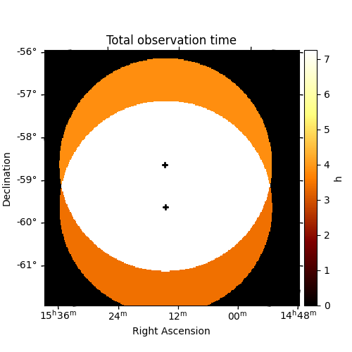
No. of observations: 17
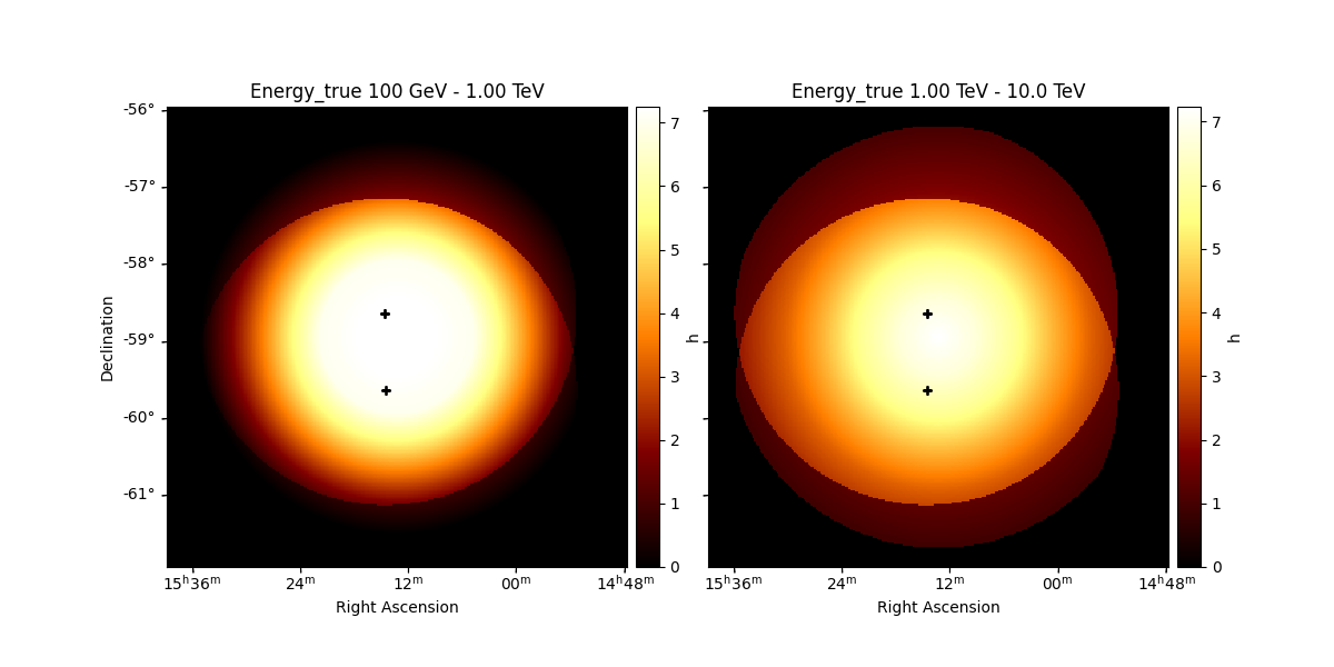
As the acceptance of IACT cameras vary within the field of view, it can also be interesting to plot the on-axis equivalent number of hours.
effective_livetime = make_effective_livetime_map(
    observations, geom, offset_max=offset_max
)


axs = effective_livetime.plot_grid(add_cbar=True)
# Add the pointing position on top
for ax in axs:
    for obs in observations:
        ax.plot(
            obs.get_pointing_icrs(obs.tmid).to_pixel(wcs=ax.wcs)[0],
            obs.get_pointing_icrs(obs.tmid).to_pixel(wcs=ax.wcs)[1],
            "+",
            color="black",
        )
plt.show()
To get the value of the observation time at a particular position,
use get_by_coord
obs_time_src = total_obstime.get_by_coord(source_pos)
effective_times_src = effective_livetime.get_by_coord(
    (source_pos, energy_axis_true.center)
)

print(f"Time spent on position {source_pos}")
print(f"Total observation time: {obs_time_src}* {total_obstime.unit}")
print(
    f"Effective livetime at {energy_axis_true.center[0]}: {effective_times_src[0]} * {effective_livetime.unit}"
)
print(
    f"Effective livetime at {energy_axis_true.center[1]}: {effective_times_src[1]} * {effective_livetime.unit}"
)
Time spent on position <SkyCoord (ICRS): (ra, dec) in deg
    (228.32, -59.08)>
Total observation time: [7.250185]* h
Effective livetime at 0.316227766016838 TeV: 7.249965667724609 * h
Effective livetime at 3.1622776601683795 TeV: 7.234359264373779 * h
Total running time of the script: (0 minutes 14.658 seconds)