Morphological energy dependence estimation

Learn how to test for energy-dependent morphology in your dataset.

Prerequisites

Knowledge on data reduction and datasets used in Gammapy, for example see the H.E.S.S. with Gammapy and Ring background map tutorials.

Context

This tutorial introduces a method to investigate the potential of energy-dependent morphology from spatial maps. It is possible for gamma-ray sources to exhibit energy-dependent morphology, in which the spatial morphology of the gamma rays varies across different energy bands. This is plausible for different source types, including pulsar wind nebulae (PWNe) and supernova remnants. HESS J1825−137 is a well-known example of a PWNe which shows a clear energy-dependent gamma-ray morphology (see Aharonian et al., 2006, H.E.S.S. Collaboration et al., 2019 and Principe et al., 2020.)

Many different techniques of measuring this energy-dependence have been utilised over the years. The method shown here is to perform a morphological fit of extension and position in various energy slices and compare this with a global morphology fit.

Objective: Perform an energy-dependent morphology study of a mock source.

Tutorial overview

This tutorial consists of two main steps.

Firstly, the user defines the initial SkyModel based on previous investigations and selects the energy bands of interest to test for energy dependence. The null hypothesis is defined as only the background component being free (norm). The alternative hypothesis introduces the source model. The results of this first step show the significance of the source above the background in each energy band.

The second step is to quantify any energy-dependent morphology. The null hypothesis is determined by performing a joint fit of the parameters. In the alternative hypothesis, the free parameters of the model are fit individually within each energy band.

Setup

from astropy import units as u
from astropy.coordinates import SkyCoord
from astropy.table import Table
import matplotlib.pyplot as plt
from IPython.display import display
from gammapy.datasets import Datasets, MapDataset
from gammapy.estimators import EnergyDependentMorphologyEstimator
from gammapy.estimators.energydependentmorphology import weighted_chi2_parameter
from gammapy.maps import Map
from gammapy.modeling.models import (
    GaussianSpatialModel,
    PowerLawSpectralModel,
    SkyModel,
)
from gammapy.stats.utils import ts_to_sigma
from gammapy.utils.check import check_tutorials_setup

Check setup

check_tutorials_setup()

System:

        python_executable      : /home/runner/work/gammapy-docs/gammapy-docs/gammapy/.tox/build_docs/bin/python
        python_version         : 3.9.19
        machine                : x86_64
        system                 : Linux


Gammapy package:

        version                : 1.3.dev198+g3e7db144f
        path                   : /home/runner/work/gammapy-docs/gammapy-docs/gammapy/.tox/build_docs/lib/python3.9/site-packages/gammapy


Other packages:

        numpy                  : 1.26.4
        scipy                  : 1.13.0
        astropy                : 5.2.2
        regions                : 0.8
        click                  : 8.1.7
        yaml                   : 6.0.1
        IPython                : 8.18.1
        jupyterlab             : not installed
        matplotlib             : 3.8.4
        pandas                 : not installed
        healpy                 : 1.16.6
        iminuit                : 2.25.2
        sherpa                 : 4.16.0
        naima                  : 0.10.0
        emcee                  : 3.1.6
        corner                 : 2.2.2
        ray                    : 2.12.0


Gammapy environment variables:

        GAMMAPY_DATA           : /home/runner/work/gammapy-docs/gammapy-docs/gammapy-datasets/dev

Obtain the data to use

Utilise the pre-defined dataset within $GAMMAPY_DATA.

P.S.: do not forget to set up your environment variable $GAMMAPY_DATA to your local directory.

stacked_dataset = MapDataset.read(
    "$GAMMAPY_DATA/estimators/mock_DL4/dataset_energy_dependent.fits.gz"
)
datasets = Datasets([stacked_dataset])

Define the energy edges of interest. These will be utilised to investigate the potential of energy-dependent morphology in the dataset.

energy_edges = [1, 3, 5, 20] * u.TeV

Define the spectral and spatial models of interest. We utilise a PowerLawSpectralModel and a GaussianSpatialModel to test the energy-dependent morphology component in each energy band. A standard 3D fit (see the 3D detailed analysis tutorial) is performed, then the best fit model is utilised here for the initial parameters in each model.

source_position = SkyCoord(5.58, 0.2, unit="deg", frame="galactic")

spectral_model = PowerLawSpectralModel(
    index=2.5, amplitude=9.8e-12 * u.Unit("cm-2 s-1 TeV-1"), reference=1.0 * u.TeV
)

spatial_model = GaussianSpatialModel(
    lon_0=source_position.l,
    lat_0=source_position.b,
    frame="galactic",
    sigma=0.2 * u.deg,
)

# Limit the search for the position on the spatial model
spatial_model.lon_0.min = source_position.galactic.l.deg - 0.8
spatial_model.lon_0.max = source_position.galactic.l.deg + 0.8
spatial_model.lat_0.min = source_position.galactic.b.deg - 0.8
spatial_model.lat_0.max = source_position.galactic.b.deg + 0.8

model = SkyModel(spatial_model=spatial_model, spectral_model=spectral_model, name="src")

Run Estimator

We can now run the energy-dependent estimation tool and explore the results.

Let’s start with the initial hypothesis, in which the source is introduced to compare with the background. We specify which parameters we wish to use for testing the energy dependence. To test for the energy dependence, it is recommended to keep the position and extension parameters free. This allows them to be used for fitting the spatial model in each energy band.

model.spatial_model.lon_0.frozen = False
model.spatial_model.lat_0.frozen = False
model.spatial_model.sigma.frozen = False

model.spectral_model.amplitude.frozen = False
model.spectral_model.index.frozen = True

datasets.models = model

estimator = EnergyDependentMorphologyEstimator(energy_edges=energy_edges, source="src")

Show the results tables

The results of the source signal above the background in each energy bin

Firstly, the estimator is run to produce the results. The table here shows the ∆(TS) value, the number of degrees of freedom (df) and the significance (σ) in each energy bin. The significance values here show that each energy band has significant signal above the background.

results = estimator.run(datasets)
table_bkg_src = Table(results["src_above_bkg"])
display(table_bkg_src)

Emin Emax      delta_ts      df    significance
TeV  TeV
---- ---- ----------------- --- ------------------
 1.0  3.0 998.0521842481248   4 31.277522957147003
 3.0  5.0  712.873581766271   4  26.34613004113985
 5.0 20.0   290.41405230487   4  16.56413952067279

The results for testing energy dependence

Next, the results of the energy-dependent estimator are shown. The table shows the various free parameters for the joint fit for \(H_0\) across the entire energy band and for each energy bin shown for \(H_1\).

ts = results["energy_dependence"]["delta_ts"]
df = results["energy_dependence"]["df"]
sigma = ts_to_sigma(ts, df=df)

print(f"The delta_ts for the energy-dependent study: {ts:.3f}.")
print(f"Converting this to a significance gives: {sigma:.3f} \u03C3")

results_table = Table(results["energy_dependence"]["result"])
display(results_table)

The delta_ts for the energy-dependent study: 76.816.
Converting this to a significance gives: 7.678 σ
Hypothesis Emin Emax ...        sigma             sigma_err
           TeV  TeV  ...         deg                 deg
---------- ---- ---- ... ------------------- --------------------
        H0  1.0 20.0 ... 0.21525376976022406 0.005914854792576181
        H1  1.0  3.0 ...  0.2568720263723087 0.009431203058496632
        H1  3.0  5.0 ... 0.19735897928723367 0.008164325487530225
        H1  5.0 20.0 ... 0.13500566998758723 0.008898002182656187

The chi-squared value for each parameter of interest

We can also utilise the weighted_chi2_parameter function for each parameter.

The weighted chi-squared significance for the sigma, lat_0 and lon_0 values.

display(
    Table(
        weighted_chi2_parameter(
            results["energy_dependence"]["result"],
            parameters=["sigma", "lat_0", "lon_0"],
        )
    )
)

parameter        chi2         df    significance
--------- ------------------ --- ------------------
    sigma  88.56393115380234   2   9.14671140315352
    lat_0  4.690311850083152   2 1.6654036168695552
    lon_0 1.3035897658854436   2  0.641635917844372

Note: The chi-squared parameter does not include potential correlation between the parameters, so it should be used cautiously.

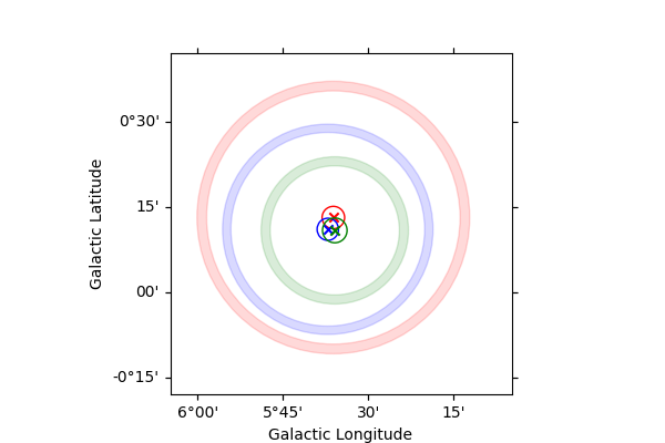
Plotting the results

empty_map = Map.create(
    skydir=spatial_model.position, frame=spatial_model.frame, width=1, binsz=0.02
)

colors = ["red", "blue", "green", "magenta"]

fig = plt.figure(figsize=(6, 4))
ax = empty_map.plot()

lat_0 = results["energy_dependence"]["result"]["lat_0"][1:]
lat_0_err = results["energy_dependence"]["result"]["lat_0_err"][1:]
lon_0 = results["energy_dependence"]["result"]["lon_0"][1:]
lon_0_err = results["energy_dependence"]["result"]["lon_0_err"][1:]
sigma = results["energy_dependence"]["result"]["sigma"][1:]
sigma_err = results["energy_dependence"]["result"]["sigma_err"][1:]

for i in range(len(lat_0)):
    model_plot = GaussianSpatialModel(
        lat_0=lat_0[i], lon_0=lon_0[i], sigma=sigma[i], frame=spatial_model.frame
    )
    model_plot.lat_0.error = lat_0_err[i]
    model_plot.lon_0.error = lon_0_err[i]
    model_plot.sigma.error = sigma_err[i]

    model_plot.plot_error(
        ax=ax,
        which="all",
        kwargs_extension={"facecolor": colors[i], "edgecolor": colors[i]},
        kwargs_position={"color": colors[i]},
    )
plt.show()


# sphinx_gallery_thumbnail_number = 1