Note
Go to the end to download the full example code. or to run this example in your browser via Binder
Priors#
Learn how you can include prior knowledge into the fitting by setting priors on single parameters.
Prerequisites#
Knowledge of spectral analysis to produce 1D spectral datasets, see the Spectral analysis tutorial.
Knowledge of fitting models to datasets, see Fitting tutorial
General knowledge of statistics and priors
Context#
Generally, the set of parameters describing best the data is where the
fit statistic
A prior on the value of some of the parameters can be added to this fit statistic. The prior is again a probability density function of the model parameters and can take different forms, including Gaussian distributions, uniform distributions, etc. The prior includes information or knowledge about the dataset or the parameters of the fit.
Setting priors on multiple parameters simultaneously is supported, However, for now, they should not be correlated.
The spectral dataset used here contains a simulated power-law source and its IRFs are based on H.E.S.S. data of the Crab Nebula (similar to Fitting). We are simulating the source here, so that we can control the input and check the correctness of the fit results.
The tutorial addresses three examples:
Including prior information about the sources index
Encouraging positive amplitude values
How to add a custom prior class?
In the first example, the Gaussian prior is used. It is shown how to set a prior on a model parameter and how it modifies the fit statistics. A source is simulated without statistics and fitted with and without the priors. The different fit results are discussed.
For the second example, 1000 datasets containing a very weak source are simulated. Due to the statistical fluctuations, the amplitude’s best-fit value is negative for some draws. By setting a uniform prior on the amplitude, this can be avoided.
The setup#
import numpy as np
from astropy import units as u
import matplotlib.pyplot as plt
from gammapy.datasets import SpectrumDatasetOnOff
from gammapy.modeling import Fit
from gammapy.modeling.models import (
    GaussianPrior,
    PowerLawSpectralModel,
    SkyModel,
    UniformPrior,
)
from gammapy.utils.check import check_tutorials_setup
Check setup#
check_tutorials_setup()
System:

        python_executable      : /home/runner/work/gammapy-docs/gammapy-docs/gammapy/.tox/build_docs/bin/python
        python_version         : 3.9.22
        machine                : x86_64
        system                 : Linux


Gammapy package:

        version                : 2.0.dev1166+g47b6a2f52
        path                   : /home/runner/work/gammapy-docs/gammapy-docs/gammapy/.tox/build_docs/lib/python3.9/site-packages/gammapy


Other packages:

        numpy                  : 1.26.4
        scipy                  : 1.13.1
        astropy                : 6.0.1
        regions                : 0.8
        click                  : 8.1.8
        yaml                   : 6.0.2
        IPython                : 8.18.1
        jupyterlab             : not installed
        matplotlib             : 3.9.4
        pandas                 : not installed
        healpy                 : 1.17.3
        iminuit                : 2.31.1
        sherpa                 : 4.16.1
        naima                  : 0.10.0
        emcee                  : 3.1.6
        corner                 : 2.2.3
        ray                    : 2.46.0


Gammapy environment variables:

        GAMMAPY_DATA           : /home/runner/work/gammapy-docs/gammapy-docs/gammapy-datasets/dev
Model and dataset#
First, we define the source model, a power-law with an index of
pl_spectrum = PowerLawSpectralModel(
    index=2.3,
    amplitude=1e-11 / u.cm**2 / u.s / u.TeV,
)
model = SkyModel(spectral_model=pl_spectrum, name="simu-source")
The data and background are read from pre-computed ON/OFF datasets of
H.E.S.S. observations. For simplicity, we stack them together and transform
the dataset to a SpectrumDataset. Then we set the model and create
an Asimov dataset (dataset without statistics) by setting the counts as
the model predictions.
dataset = SpectrumDatasetOnOff.read(
    "$GAMMAPY_DATA/joint-crab/spectra/hess/pha_obs23523.fits"
)

# Set model and fit range
e_min = 0.66 * u.TeV
e_max = 30 * u.TeV
dataset.mask_fit = dataset.counts.geom.energy_mask(e_min, e_max)
dataset = dataset.to_spectrum_dataset()

dataset1 = dataset.copy()
dataset1.models = model.copy(name="model")
dataset1.counts = dataset1.npred()
Example 1: Including Prior Information about the Sources Index#
The index was assumed to be
# initialising the gaussian prior
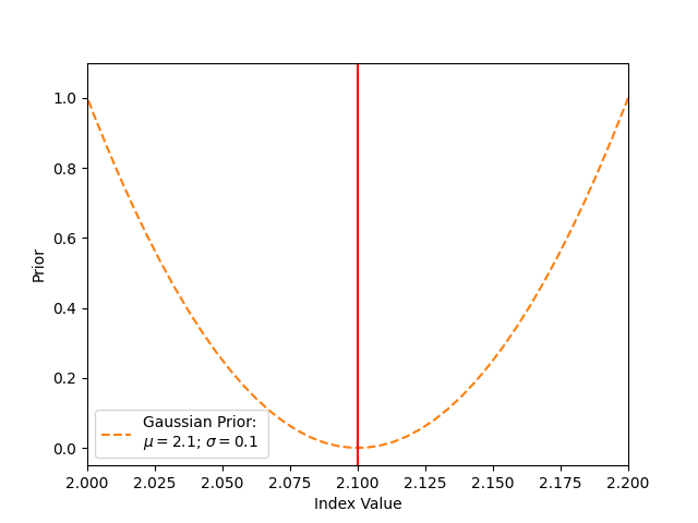
gaussianprior = GaussianPrior(mu=2.1, sigma=0.1)
# setting the gaussian prior on the index parameter
model_prior = model.copy()
model_prior.parameters["index"].prior = gaussianprior
The value of the prior depends on the value of the index. If the index value equals the Gaussians mean (here 2.1), the prior is zero. This means that nothing is added to the cash statistics, and this value is favoured in the fit. If the value of the index deviates from the mean of 2.1, a prior value > 0 is added to the cash statistics.
# For the visualisation, the values are appended to the list; this is not a necessity for the fitting
prior_stat_sums = []
with model_prior.parameters.restore_status():
    i_scan = np.linspace(1.8, 2.3, 100)
    for a in i_scan:
        model_prior.parameters["index"].value = a
        prior_stat_sums.append(model_prior.parameters.prior_stat_sum())

plt.plot(
    i_scan,
    prior_stat_sums,
    color="tab:orange",
    linestyle="dashed",
    label=f"Gaussian Prior: \n$\mu = {gaussianprior.mu.value}$; $\sigma = {gaussianprior.sigma.value}$",
)
plt.axvline(x=gaussianprior.mu.value, color="red")

plt.xlabel("Index Value")
plt.ylabel("Prior")
plt.legend()
plt.xlim(2.0, 2.2)
plt.ylim(-0.05, 1.1)
plt.show()
Fitting a Dataset with and without the Prior#
Now, we copy the dataset consisting of the power-law source and assign the model with the Gaussian prior set on its index to it. Both of the datasets are fitted.
dataset1.fake()
dataset1_prior = dataset1.copy()
dataset1_prior.models = model_prior.copy(name="prior-model")

fit = Fit()
results = fit.run(dataset1)

results_prior = fit.run(dataset1_prior)
The parameters table will mention the type of prior associated to each model
   model    type    name     value    ... max frozen link     prior
----------- ---- --------- ---------- ... --- ------ ---- -------------
prior-model          index 2.1211e+00 ... nan  False      GaussianPrior
prior-model      amplitude 9.0030e-12 ... nan  False
prior-model      reference 1.0000e+00 ... nan   True
To see the details of the priors, eg:
print(results_prior.models.parameters["index"].prior)
GaussianPrior

 type  name   value    unit   error   min max
----- ----- ---------- ---- --------- --- ---
prior    mu 2.1000e+00      0.000e+00 nan nan
prior sigma 1.0000e-01      0.000e+00 nan nan
The Likelihood profiles can be computed for both the datasets. Hereby, the likelihood gets computed for different values of the index. For each step the other free parameters are getting reoptimized.
dataset1.models.parameters["index"].scan_n_values = 20
dataset1_prior.models.parameters["index"].scan_n_values = 20

scan = fit.stat_profile(datasets=dataset1, parameter="index", reoptimize=True)

scan_prior = fit.stat_profile(
    datasets=dataset1_prior, parameter="index", reoptimize=True
)
Now, we can compare the two Likelihood scans. In the first case, we did
not set any prior. This means that only the Cash Statistic itself is
getting minimized. The Cash statistics minimum is the actual value of
the index we used for the simulation (
The plot also shows the prior we set on the index for the second
dataset. The scan was computed above. If the logarithm of the prior is added to the cash
statistics, one ends up with the posterior function. The posterior is
minimized during the second fit to obtain the maximum a posteriori estimation. Its minimum is between the priors and
the cash statistics minimum. The best-fit value is
The best-fit index value and uncertainty depend strongly on the standard
deviation of the Gaussian prior. You can vary
plt.plot(scan["model.spectral.index_scan"], scan["stat_scan"], label="Cash Statistics")
plt.plot(
    i_scan,
    np.array(prior_stat_sums) + np.min(scan["stat_scan"]),
    linestyle="dashed",
    label="Prior",
)
plt.plot(
    scan_prior["prior-model.spectral.index_scan"],
    scan_prior["stat_scan"],
    label="Posterior\n(Cash Stat. + Prior)",
)

par = dataset1.models.parameters["index"]
plt.errorbar(
    x=par.value,
    y=np.min(scan["stat_scan"]) + 1,
    xerr=par.error,
    fmt="x",
    markersize=6,
    capsize=8,
    color="darkblue",
    label="Best-Fit w/o Prior",
)
par = dataset1_prior.models.parameters["index"]
plt.errorbar(
    x=par.value,
    y=np.min(scan_prior["stat_scan"]) + 1,
    xerr=par.error,
    fmt="x",
    markersize=6,
    capsize=8,
    color="darkgreen",
    label="Best-Fit w/ Prior",
)
plt.legend()
# plt.ylim(31.5,35)
plt.xlabel("Index")
plt.ylabel("Fit Statistics [arb. unit]")
plt.show()
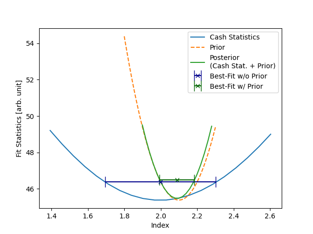
This example shows a critical note on using priors: we were able to manipulate the best-fit index. This can have multiple advantages if one wants to include additional information. But it should always be used carefully to not falsify or bias any results!
Note how the
Example 2: Encouraging Positive Amplitude Values#
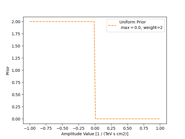
In the next example, we want to encourage the amplitude to have positive, i.e. physical, values. Instead of setting hard bounds, we can also set a uniform prior, which prefers positive values to negatives.
We set the amplitude of the power-law used to simulate the source to a very small value. Together with statistical fluctuations, this could result in some negative amplitude best-fit values.
model_weak = SkyModel(
    PowerLawSpectralModel(
        amplitude=1e-13 / u.cm**2 / u.s / u.TeV,
    ),
    name="weak-model",
)
model_weak_prior = model_weak.copy(name="weak-model-prior")
uniform = UniformPrior(min=0)
uniform.weight = 2
model_weak_prior.parameters["amplitude"].prior = uniform
We set the minimum value to zero and per default, the maximum value is set to positive infinity. Therefore, the uniform prior penalty is zero, i.e. no influence on the fit at all, if the amplitude value is positive and a penalty (the weight) in the form of a prior likelihood for negative values. Here, we are setting it to 2. This value is only applied if the amplitude value goes below zero.
uni_prior_stat_sums = []
with model_weak_prior.parameters.restore_status():
    a_scan = np.linspace(-1, 1, 100)
    for a in a_scan:
        model_weak_prior.parameters["amplitude"].value = a
        uni_prior_stat_sums.append(model_weak_prior.parameters.prior_stat_sum())

plt.plot(
    a_scan,
    uni_prior_stat_sums,
    color="tab:orange",
    linestyle="dashed",
    label=f"Uniform Prior\n $min={uniform.min.value}$, weight={uniform.weight}",
)
plt.xlabel("Amplitude Value [1 / (TeV s cm2)]")
plt.ylabel("Prior")
plt.legend()
plt.show()
Fitting Multiple Datasets with and without the Prior#
To showcase how the uniform prior affects the fit results,
results, results_prior = [], []
N = 100
dataset2 = dataset.copy()
for n in range(N):
    # simulating the dataset
    dataset2.models = model_weak.copy()
    dataset2.fake()

    dataset2_prior = dataset2.copy()
    dataset2_prior.models = model_weak_prior.copy()
    # fitting without the prior
    fit = Fit()
    result = fit.optimize(dataset2)
    results.append(
        {
            "index": result.parameters["index"].value,
            "amplitude": result.parameters["amplitude"].value,
        }
    )
    # fitting with the prior
    fit_prior = Fit()
    result = fit_prior.optimize(dataset2_prior)
    results_prior.append(
        {
            "index": result.parameters["index"].value,
            "amplitude": result.parameters["amplitude"].value,
        }
    )


fig, axs = plt.subplots(1, 2, figsize=(7, 4))
for i, parname in enumerate(["index", "amplitude"]):
    par = np.array([_[parname] for _ in results])
    c, bins, _ = axs[i].hist(par, bins=20, alpha=0.5, label="Without Prior")
    par = np.array([_[parname] for _ in results_prior])
    axs[i].hist(par, bins=bins, alpha=0.5, color="tab:green", label="With Prior")
    axs[i].axvline(x=model_weak.parameters[parname].value, color="red")
    axs[i].set_xlabel(f"Reconstructed spectral\n {parname}")
    axs[i].legend()
plt.tight_layout()
plt.show()
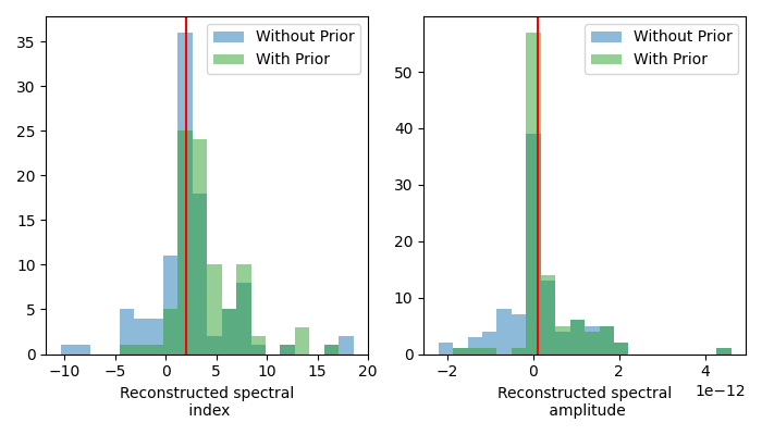
The distribution of the best-fit amplitudes shows how less best-fit amplitudes have negative values. This also has an effect on the distribution of the best-fit indices. How exactly the distribution changes depends on the weight assigned to the uniform prior. The stronger the weight, the less negative amplitudes.
Note that the model parameters uncertainties are, per default, computed symmetrical. This can lead to incorrect uncertainties, especially with asymmetrical priors like the previous uniform. Calculating the uncertainties from the profile likelihood is advised. For more details see the Fitting tutorial.
Implementing a custom prior#
For now, only GaussianPrior and UniformPrior are implemented.
To add a use case specific prior one has to create a prior subclass
containing:
a tag and a _type used for the serialization
an instantiation of each PriorParameter with their unit and default values
the evaluate function where the mathematical expression for the prior is defined.
As an example for a custom prior a Jeffrey prior for a scale parameter is chosen.
The only parameter is sigma and the evaluation method return the squared inverse of sigma.
from gammapy.modeling import PriorParameter
from gammapy.modeling.models import Model, Prior


class MyCustomPrior(Prior):
    """Custom Prior.


    Parameters
    ----------
    min : float
        Minimum value.
        Default is -inf.
    max : float
        Maximum value.
        Default is inf.
    """

    tag = ["MyCustomPrior"]
    sigma = PriorParameter(name="sigma", value=1, unit="")
    _type = "prior"

    @staticmethod
    def evaluate(value, sigma):
        """Evaluate the custom prior."""
        return value / sigma**2


# The custom prior is added to the PRIOR_REGISTRY so that it can be serialised.

from gammapy.modeling.models import PRIOR_REGISTRY

PRIOR_REGISTRY.append(MyCustomPrior)

# The custom prior is set on the index of a powerlaw spectral model and is evaluated.
customprior = MyCustomPrior(sigma=0.5)
pwl = PowerLawSpectralModel()
pwl.parameters["index"].prior = customprior
customprior(pwl.parameters["index"])

# The power law spectral model can be written into a dictionary.
# If a model is read in from this dictionary, the custom prior is still set on the index.

print(pwl.to_dict())
model_read = Model.from_dict(pwl.to_dict())
model_read.parameters.prior
{'spectral': {'type': 'PowerLawSpectralModel', 'parameters': [{'name': 'index', 'value': 2.0, 'prior': {'type': 'MyCustomPrior', 'parameters': [{'name': 'sigma', 'value': 0.5, 'unit': ''}], 'weight': 1}}, {'name': 'amplitude', 'value': 1e-12, 'unit': 'TeV-1 s-1 cm-2'}, {'name': 'reference', 'value': 1.0, 'unit': 'TeV'}]}}

[<__main__.MyCustomPrior object at 0x7f3eb5291be0>, None, None]
Total running time of the script: (1 minutes 2.783 seconds)