Note
Go to the end to download the full example code. or to run this example in your browser via Binder
Estimators#
This tutorial provides an overview of the Estimator API. All estimators live in the
gammapy.estimators sub-module, offering a range of algorithms and classes for high-level flux and
significance estimation. This is accomplished through a common functionality allowing the estimation of
flux points, light curves, flux maps and profiles via a common API.
Key Features#
Hypothesis Testing: Estimations are based on testing a reference model against a null hypothesis, deriving flux and significance values.
Estimation via Two Methods:
Model Fitting (Forward Folding): Refit the flux of a model component within specified energy, time, or spatial regions.
Excess Calculation (Backward Folding): Use the analytical solution by Li and Ma for significance based on excess counts, currently available in
ExcessMapEstimator.
For further information on these details please refer to Estimators (DL4 to DL5, and DL6).
The setup#
import numpy as np
import matplotlib.pyplot as plt
from astropy import units as u
from IPython.display import display
from gammapy.datasets import SpectrumDatasetOnOff, Datasets, MapDataset
from gammapy.estimators import (
    FluxPointsEstimator,
    ExcessMapEstimator,
    FluxPoints,
)
from gammapy.modeling import Fit, Parameter
from gammapy.modeling.models import SkyModel, PowerLawSpectralModel
from gammapy.utils.scripts import make_path
Flux Points Estimation#
We start with a simple example for flux points estimation taking multiple datasets into account.
In this section we show the steps to estimate the flux points.
First we read the pre-computed datasets from $GAMMAPY_DATA.
Next we define a spectral model and set it on the datasets:
pwl = PowerLawSpectralModel(index=2.7, amplitude="5e-11  cm-2 s-1 TeV-1")
datasets.models = SkyModel(spectral_model=pwl, name="crab")
Before using the estimators, it is necessary to first ensure that the model is properly fitted. This applies to all scenarios, including light curve estimation. To optimize the model parameters to best fit the data we utilise the following:
fit = Fit()
fit_result = fit.optimize(datasets=datasets)
print(fit_result)
OptimizeResult

        backend    : minuit
        method     : migrad
        success    : True
        message    : Optimization terminated successfully.
        nfev       : 37
        total stat : 156.99
A fully configured Flux Points Estimation#
The FluxPointsEstimator estimates flux points for a given list of datasets,
energies and spectral model. The most simple way to call the estimator is by defining both
the name of the source and its energy_edges.
Here we prepare a full configuration of the flux point estimation.
Firstly we define the backend for the fit:
Define the fully configured flux points estimator:
energy_edges = np.geomspace(0.7, 100, 9) * u.TeV
norm = Parameter(name="norm", value=1.0)

fp_estimator = FluxPointsEstimator(
    source="crab",
    energy_edges=energy_edges,
    n_sigma=1,
    n_sigma_ul=2,
    selection_optional="all",
    fit=fit,
    norm=norm,
)
The norm parameter can be adjusted in a few different ways. For example, we can change its
minimum and maximum values that it scans over, as follows.
Note: The default scan range of the norm parameter is between 0.2 to 5. In case the upper limit values lie outside this range, nan values will be returned. It may thus be useful to increase this range, specially for the computation of upper limits from weak sources.
The various quantities utilised in this tutorial are described here:
source: which source from the model to compute the flux points forenergy_edges: edges of the flux points energy binsn_sigma: number of sigma for the flux errorn_sigma_ul: the number of sigma for the flux upper limitsselection_optional: what additional maps to computefit: the fit instance (as defined above)reoptimize: whether to reoptimize the flux points with other model parameters, aside from thenormnorm: normalisation parameter for the fit
Important note: the output energy_edges are taken from the parent dataset energy bins,
selecting the bins closest to the requested energy_edges. To match the input bins directly,
specific binning must be defined based on the parent dataset geometry. This could be done in the following way:
energy_edges = datasets[0].geoms["geom"].axes["energy"].downsample(factor=5).edges
Accessing and visualising the results#
print(fp_result)
FluxPoints
----------

  geom                   : RegionGeom
  axes                   : ['lon', 'lat', 'energy']
  shape                  : (1, 1, 8)
  quantities             : ['norm', 'norm_err', 'norm_errn', 'norm_errp', 'norm_ul', 'norm_sensitivity', 'ts', 'npred', 'npred_excess', 'stat', 'stat_null', 'stat_scan', 'counts', 'success']
  ref. model             : pl
  n_sigma                : 1
  n_sigma_ul             : 2
  sqrt_ts_threshold_ul   : 2
  sed type init          : likelihood
We can specify the SED type to plot:
fp_result.plot(sed_type="dnde")
plt.show()
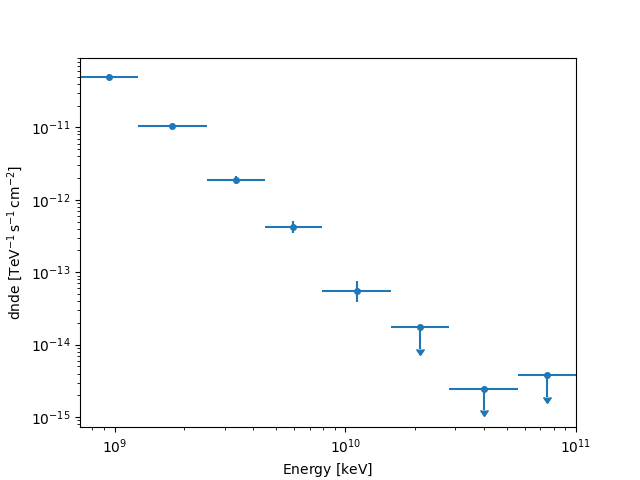
We can also access
the quantities names through fp_result.available_quantities.
Here we show how you can plot a different plot type and define the axes units,
we also overlay the TS profile.
ax = plt.subplot()
ax.xaxis.set_units(u.eV)
ax.yaxis.set_units(u.Unit("TeV cm-2 s-1"))
fp_result.plot(ax=ax, sed_type="e2dnde", color="tab:orange")
fp_result.plot_ts_profiles(sed_type="e2dnde")
plt.show()
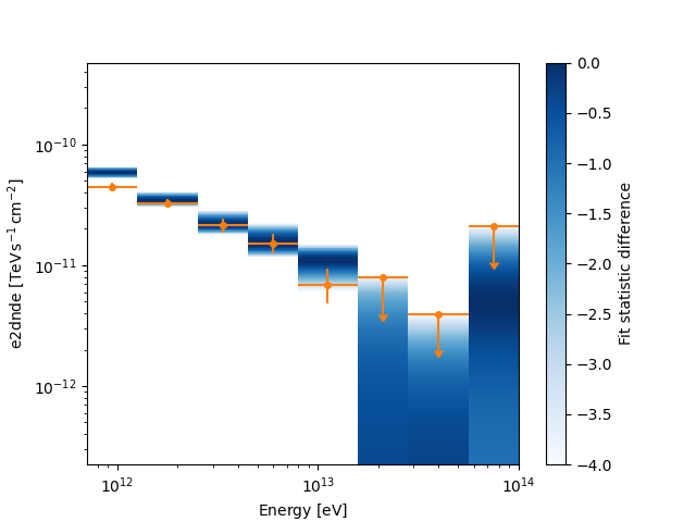
The actual data members are N-dimensional RegionNDMap objects. So you can
also plot them:
print(type(fp_result.dnde))
<class 'gammapy.maps.region.ndmap.RegionNDMap'>
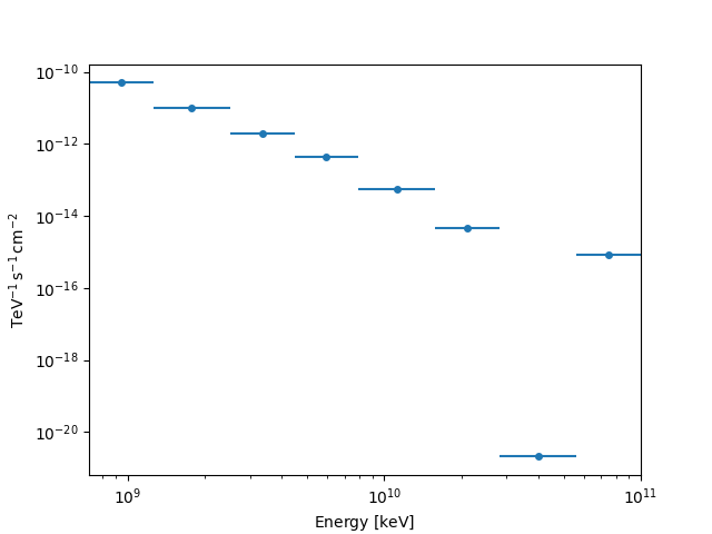
From the above, we can see that we access to many quantities.
Access the data:
print(fp_result.e2dnde.quantity.to("TeV cm-2 s-1"))
[[[ 4.45517415e-11]]

 [[ 3.25823909e-11]]

 [[ 2.13944023e-11]]

 [[ 1.51958055e-11]]

 [[ 6.92052435e-12]]

 [[ 2.03447394e-12]]

 [[-7.72411791e-28]]

 [[ 4.71359513e-12]]] TeV / (s cm2)
(8, 1, 1)
print(fp_result.dnde.quantity[:, 0, 0])
[ 4.99878762e-11  1.03034567e-11  1.90677811e-12  4.28275990e-13
  5.49716789e-14  4.55461982e-15 -4.87358893e-31  8.38208917e-16] 1 / (TeV s cm2)
Or even extract an energy range:
fp_result.dnde.slice_by_idx({"energy": slice(3, 10)})
A note on the internal representation#
The result contains a reference spectral model, which defines the spectral shape. Typically, it is the best fit model:
print(fp_result.reference_model)
SkyModel

  Name                      : fyhK0OXp
  Datasets names            : None
  Spectral model type       : PowerLawSpectralModel
  Spatial  model type       :
  Temporal model type       :
  Parameters:
    index                         :      2.700   +/-    0.00
    amplitude                     :   4.58e-11   +/- 0.0e+00 1 / (TeV s cm2)
    reference             (frozen):      1.000       TeV
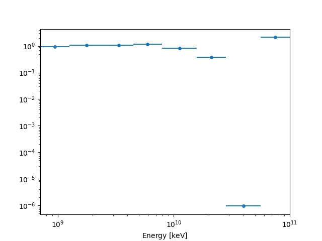
FluxPoints are the represented by the “norm” scaling factor with
respect to the reference model:
Dataset specific quantities (“counts like”)#
While the flux estimate and associated errors are common to all datasets, the result also stores some dataset specific quantities, which can be useful for debugging. Here we remind the user of the meaning of the forthcoming quantities:
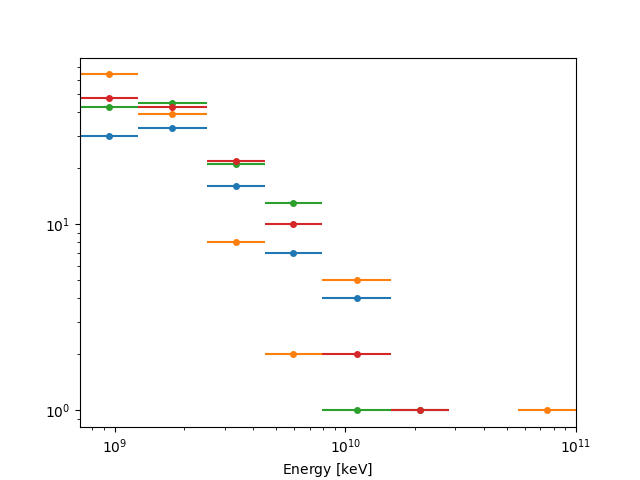
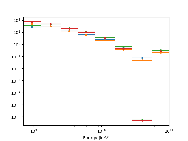
counts: predicted counts from the null hypothesis,npred: predicted number of counts from best fit hypothesis,npred_excess: predicted number of excess counts from best fit hypothesis.
The RegionNDMap allows for plotting of multidimensional data
as well, by specifying the primary axis_name:
fp_result.counts.plot(axis_name="energy")
plt.show()
fp_result.npred.plot(axis_name="energy")
plt.show()
fp_result.npred_excess.plot(axis_name="energy")
plt.show()
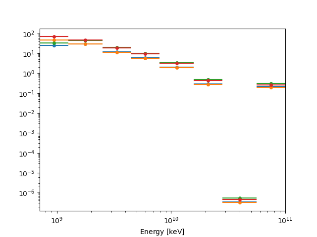
Table conversion#
Flux points can be converted to tables:
table = fp_result.to_table(sed_type="flux", format="gadf-sed")
display(table)
      e_ref              e_min              e_max        ... success  norm_scan
       keV                keV                keV         ...
------------------ ------------------ ------------------ ... ------- -----------
 944060876.2859229  707945784.3841385 1258925411.7941697 ...    True 0.1 .. 10.0
  1778279410.03893 1258925411.7941697  2511886431.509587 ...    True 0.1 .. 10.0
3349654391.5782814  2511886431.509587  4466835921.509632 ...    True 0.1 .. 10.0
 5956621435.290098  4466835921.509632 7943282347.2428255 ...    True 0.1 .. 10.0
11220184543.019672 7943282347.2428255 15848931924.611168 ...    True 0.1 .. 10.0
21134890398.366486 15848931924.611168 28183829312.644527 ...    True 0.1 .. 10.0
39810717055.349655 28183829312.644527  56234132519.03493 ...    True 0.1 .. 10.0
 74989420933.24579  56234132519.03493 100000000000.00015 ...    True 0.1 .. 10.0
table = fp_result.to_table(sed_type="likelihood", format="gadf-sed", formatted=True)
display(table)
     e_ref           e_min           e_max       ... success    norm_scan
      keV             keV             keV        ...
--------------- --------------- ---------------- ... ------- ---------------
  944060876.286   707945784.384   1258925411.794 ...    True 0.100 .. 10.000
 1778279410.039  1258925411.794   2511886431.510 ...    True 0.100 .. 10.000
 3349654391.578  2511886431.510   4466835921.510 ...    True 0.100 .. 10.000
 5956621435.290  4466835921.510   7943282347.243 ...    True 0.100 .. 10.000
11220184543.020  7943282347.243  15848931924.611 ...    True 0.100 .. 10.000
21134890398.366 15848931924.611  28183829312.645 ...    True 0.100 .. 10.000
39810717055.350 28183829312.645  56234132519.035 ...    True 0.100 .. 10.000
74989420933.246 56234132519.035 100000000000.000 ...    True 0.100 .. 10.000
Common API#
In GAMMAPY_DATA we have access to other FluxPoints objects
which have been created utilising the above method. Here we read the PKS 2155-304 light curve
and create a FluxMaps object and show the data structure of such objects.
We emphasize that these follow a very similar structure.
Load the light curve for the PKS 2155-304 as a FluxPoints object.#
lightcurve = FluxPoints.read(
    "$GAMMAPY_DATA/estimators/pks2155_hess_lc/pks2155_hess_lc.fits", format="lightcurve"
)

display(lightcurve.available_quantities)
['norm', 'norm_err', 'norm_errn', 'norm_errp', 'norm_ul', 'ts', 'sqrt_ts', 'npred', 'npred_excess', 'stat', 'stat_null', 'stat_scan', 'is_ul', 'counts', 'success']
Create a FluxMaps object through one of the estimators.#
dataset = MapDataset.read("$GAMMAPY_DATA/cta-1dc-gc/cta-1dc-gc.fits.gz")
estimator = ExcessMapEstimator(correlation_radius="0.1 deg")
result = estimator.run(dataset)
display(result)
FluxMaps
--------

  geom                   : WcsGeom
  axes                   : ['lon', 'lat', 'energy']
  shape                  : (320, 240, 1)
  quantities             : ['npred', 'npred_excess', 'counts', 'ts', 'sqrt_ts', 'norm', 'norm_err']
  ref. model             : pl
  n_sigma                : 1
  n_sigma_ul             : 2
  sqrt_ts_threshold_ul   : 2
  sed type init          : likelihood
display(result.available_quantities)
['npred', 'npred_excess', 'counts', 'ts', 'sqrt_ts', 'norm', 'norm_err']
Total running time of the script: (0 minutes 27.100 seconds)
