Note
Go to the end to download the full example code. or to run this example in your browser via Binder
Account for spectral absorption due to the EBL#
Gamma rays emitted from extra-galactic objects, eg blazars, interact with the photons of the Extragalactic Background Light (EBL) through pair production and are attenuated, thus modifying the intrinsic spectrum.
Various models of the EBL are supplied in GAMMAPY_DATA. This
notebook shows how to use these models to correct for this interaction.
Setup#
As usual, we’ll start with the standard imports …
import astropy.units as u
import matplotlib.pyplot as plt
from gammapy.catalog import SourceCatalog4FGL
from gammapy.datasets import SpectrumDatasetOnOff
from gammapy.estimators import FluxPointsEstimator
from gammapy.modeling import Fit
from gammapy.modeling.models import (
    EBL_DATA_BUILTIN,
    EBLAbsorptionNormSpectralModel,
    GaussianPrior,
    PowerLawSpectralModel,
    SkyModel,
)
Load the data#
We will use 6 observations of the blazars PKS 2155-304 taken in 2008 by
H.E.S.S. when it was in a steady state. The data have already been
reduced to OGIP format SpectrumDatasetOnOff following the procedure
Spectral analysis tutorial using a
ReflectedRegions background estimation. The spectra and IRFs from the
6 observations have been stacked together.
We will load this dataset as a SpectrumDatasetOnOff and proceed with
the modeling. You can do a 3D analysis as well.
dataset = SpectrumDatasetOnOff.read(
    "$GAMMAPY_DATA/PKS2155-steady/pks2155-304_steady.fits.gz"
)

print(dataset)
SpectrumDatasetOnOff
--------------------

  Name                            : stacked

  Total counts                    : 119
  Total background counts         : 37.75
  Total excess counts             : 81.25

  Predicted counts                : 44.00
  Predicted background counts     : 44.00
  Predicted excess counts         : nan

  Exposure min                    : 3.80e+05 m2 s
  Exposure max                    : 2.68e+09 m2 s

  Number of total bins            : 10
  Number of fit bins              : 8

  Fit statistic type              : wstat
  Fit statistic value (-2 log(L)) : 109.21

  Number of models                : 0
  Number of parameters            : 0
  Number of free parameters       : 0

  Total counts_off                : 453
  Acceptance                      : 8
  Acceptance off                  : 96
Model the observed spectrum#
The observed spectrum is already attenuated due to the EBL. Assuming
that the intrinsic spectrum is a power law, the observed spectrum is a
gammapy.modeling.models.CompoundSpectralModel given by the product of an EBL model with the
intrinsic model.
For a list of available models, see EBL_DATA_BUILTIN.
print(EBL_DATA_BUILTIN.keys())
dict_keys(['franceschini', 'dominguez', 'finke', 'franceschini17', 'saldana-lopez21'])
To use other EBL models, you need to save the optical depth as a function of energy and redshift as an XSPEC model. Alternatively, you can use packages like ebltable which shows how to interface other EBL models with Gammapy.
Define the power law
index = 2.3
amplitude = 1.81 * 1e-12 * u.Unit("cm-2 s-1 TeV-1")
reference = 1 * u.TeV
pwl = PowerLawSpectralModel(index=index, amplitude=amplitude, reference=reference)
pwl.index.frozen = False
# Specify the redshift of the source
redshift = 0.116

# Load the EBL model. Here we use the model from Dominguez, 2011
absorption = EBLAbsorptionNormSpectralModel.read_builtin("dominguez", redshift=redshift)


# The power-law model is multiplied by the EBL to get the final model
spectral_model = pwl * absorption
print(spectral_model)
CompoundSpectralModel
    Component 1 : PowerLawSpectralModel

type    name     value         unit        error   min max frozen link prior
---- --------- ---------- -------------- --------- --- --- ------ ---- -----
         index 2.3000e+00                0.000e+00 nan nan  False
     amplitude 1.8100e-12 TeV-1 s-1 cm-2 0.000e+00 nan nan  False
     reference 1.0000e+00            TeV 0.000e+00 nan nan   True
    Component 2 : EBLAbsorptionNormSpectralModel

type    name      value    unit   error   min max frozen link prior
---- ---------- ---------- ---- --------- --- --- ------ ---- -----
       redshift 1.1600e-01      0.000e+00 nan nan   True
     alpha_norm 1.0000e+00      0.000e+00 nan nan   True
    Operator : mul
Now, create a sky model and proceed with the fit
sky_model = SkyModel(spatial_model=None, spectral_model=spectral_model, name="pks2155")

dataset.models = sky_model
Note that since this dataset has been produced by a reflected region analysis, it uses ON-OFF statistic and does not require a background model.
fit = Fit()
result = fit.run(datasets=[dataset])

# we make a copy here to compare it later
model_best = sky_model.copy()

print(result.models.to_parameters_table())
 model  type    name      value         unit      ... min max frozen link prior
------- ---- ---------- ---------- -------------- ... --- --- ------ ---- -----
pks2155           index 2.5531e+00                ... nan nan  False
pks2155       amplitude 1.2978e-11 TeV-1 s-1 cm-2 ... nan nan  False
pks2155       reference 1.0000e+00            TeV ... nan nan   True
pks2155        redshift 1.1600e-01                ... nan nan   True
pks2155      alpha_norm 1.0000e+00                ... nan nan   True
Get the flux points#
To get the observed flux points, just run the FluxPointsEstimator
normally
energy_edges = dataset.counts.geom.axes["energy"].edges
fpe = FluxPointsEstimator(
    energy_edges=energy_edges, source="pks2155", selection_optional="all"
)
flux_points_obs = fpe.run(datasets=[dataset])
To get the deabsorbed flux points (ie, intrinsic points), we simply need to set the reference model to the best fit power law instead of the compound model.
flux_points_intrinsic = flux_points_obs.copy(
    reference_model=SkyModel(spectral_model=pwl)
)

#
print(flux_points_obs.reference_model)

#
print(flux_points_intrinsic.reference_model)
SkyModel

  Name                      : ttBnxJXx
  Datasets names            : None
  Spectral model type       : CompoundSpectralModel
  Spatial  model type       :
  Temporal model type       :
  Parameters:
    index                         :      2.553   +/-    0.30
    amplitude                     :   1.30e-11   +/- 1.9e-12 1 / (TeV s cm2)
    reference             (frozen):      1.000       TeV
    redshift              (frozen):      0.116
    alpha_norm            (frozen):      1.000


SkyModel

  Name                      : NFAn2GdN
  Datasets names            : None
  Spectral model type       : PowerLawSpectralModel
  Spatial  model type       :
  Temporal model type       :
  Parameters:
    index                         :      2.553   +/-    0.30
    amplitude                     :   1.30e-11   +/- 1.9e-12 1 / (TeV s cm2)
    reference             (frozen):      1.000       TeV
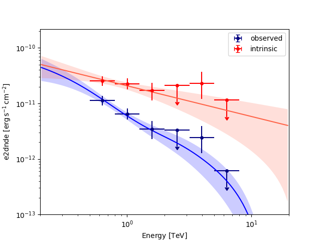
Plot the observed and intrinsic fluxes#
plt.figure()
sed_type = "e2dnde"
energy_bounds = [0.2, 20] * u.TeV
ax = flux_points_obs.plot(sed_type=sed_type, label="observed", color="navy")
flux_points_intrinsic.plot(ax=ax, sed_type=sed_type, label="intrinsic", color="red")

model_best.spectral_model.plot(
    ax=ax, energy_bounds=energy_bounds, sed_type=sed_type, color="blue"
)
model_best.spectral_model.plot_error(
    ax=ax, energy_bounds=energy_bounds, sed_type="e2dnde", facecolor="blue"
)

pwl.plot(ax=ax, energy_bounds=energy_bounds, sed_type=sed_type, color="tomato")
pwl.plot_error(
    ax=ax, energy_bounds=energy_bounds, sed_type=sed_type, facecolor="tomato"
)
plt.ylim(bottom=1e-13)
plt.legend()
plt.show()
Further extensions#
In this notebook, we have kept the parameters of the EBL model, the
alpha_norm and the redshift frozen. Under reasonable assumptions
on the intrinsic spectrum, it can be possible to constrain these
parameters.
Example: We now assume that the FermiLAT 4FGL catalog spectrum of the source is a good assumption of the intrinsic spectrum.
NOTE: This is a very simplified assumption and in reality, EBL absorption can affect the Fermi spectrum significantly. Also, blazar spectra vary with time and long term averaged states may not be representative of a specific steady state
catalog = SourceCatalog4FGL()

src = catalog["PKS 2155-304"]

# Get the intrinsic model
intrinsic_model = src.spectral_model()
print(intrinsic_model)
LogParabolaSpectralModel

type    name     value         unit        error   min max frozen link prior
---- --------- ---------- -------------- --------- --- --- ------ ---- -----
     amplitude 1.2591e-11 MeV-1 s-1 cm-2 1.317e-13 nan nan  False
     reference 1.1610e+03            MeV 0.000e+00 nan nan   True
         alpha 1.7733e+00                1.029e-02 nan nan  False
          beta 4.1893e-02                3.743e-03 nan nan  False
We add Gaussian priors on the alpha and beta parameters based on the 4FGL
measurements and the associated errors. For more details on using priors, see
Priors
As before, multiply the intrinsic model with the EBL model
Now, free the redshift of the source
obs_model.parameters["redshift"].frozen = False

print(obs_model.parameters.to_table())

sky_model = SkyModel(spectral_model=obs_model, name="observed")
dataset.models = sky_model

result1 = fit.run([dataset])

print(result1.parameters.to_table())
type    name      value         unit      ... max frozen link     prior
---- ---------- ---------- -------------- ... --- ------ ---- -------------
      amplitude 1.2591e-11 MeV-1 s-1 cm-2 ... nan  False
      reference 1.1610e+03            MeV ... nan   True
          alpha 1.7733e+00                ... nan  False      GaussianPrior
           beta 4.1893e-02                ... nan  False      GaussianPrior
       redshift 1.1600e-01                ... nan  False
     alpha_norm 1.0000e+00                ... nan   True
type    name      value         unit      ... max frozen link     prior
---- ---------- ---------- -------------- ... --- ------ ---- -------------
      amplitude 1.9692e-11 MeV-1 s-1 cm-2 ... nan  False
      reference 1.1610e+03            MeV ... nan   True
          alpha 1.7733e+00                ... nan  False      GaussianPrior
           beta 4.1896e-02                ... nan  False      GaussianPrior
       redshift 1.4338e-01                ... nan  False
     alpha_norm 1.0000e+00                ... nan   True
Get a fit stat profile for the redshift#
For more information about stat profiles, see Fitting
total_stat = result1.total_stat

par = sky_model.parameters["redshift"]
par.scan_max = par.value + 5.0 * par.error
par.scan_min = max(0, par.value - 5.0 * par.error)
par.scan_n_values = 31

# %time
profile = fit.stat_profile(
    datasets=[dataset], parameter=sky_model.parameters["redshift"], reoptimize=True
)

plt.figure()
ax = plt.gca()
ax.plot(
    profile["observed.spectral.model2.redshift_scan"], profile["stat_scan"] - total_stat
)
ax.set_title("TS profile")
ax.set_xlabel("Redshift")
ax.set_ylabel("$\Delta$ TS")
plt.show()
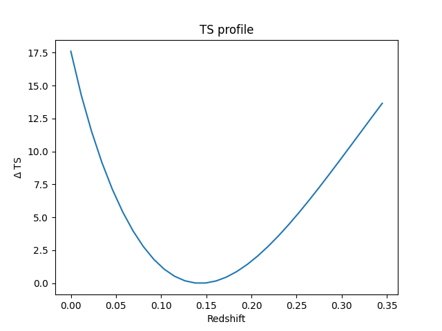
We see that the redshift is well constrained.
Total running time of the script: (0 minutes 25.353 seconds)